2 Basic R
This course is designed for people who already have a basic familiarity with R. This chapter serves as a refresher on basic concepts, and highlights some specific use cases that will be important for the way we will use R in this course.
The textbook for my intro to R class, PSCI 1800, is available here if you feel you need additional reminders about anything I don’t cover here.
There are two main things that we will be doing in R that are particular to this class that I want to refresh: generating simulations, and working with survey datasets using the tidyverse suite of packages.
2.1 R for Simulations
2.1.1 Boolean Variables
One of the “secret” powers of R is working with True or False, or “Boolean”, variables. R can easily test a large number of objects for some sort of logical condition and return a bunch of trues and falses. Further, R very helpfully treats “True” as the number 1, and “False” as the number 0, which we will see has extremely helpful mathematical properties.
If we give R some expressions that can be True or False, it will evaluate them:
2 == 1+1
#> [1] TRUE

1/2 == .5
#> [1] TRUE

2 == 3
#> [1] FALSE

2/3 == .6666
#> [1] FALSE
When we hae a vector of information that we create with concatenate (c()) we can also use the double equals sign (or any other boolean operator):
vec <- c(1,2,3,4,5)

vec == 3
#> [1] FALSE FALSE  TRUE FALSE FALSE
We can see that R went through and evaluated each of the items in vec as true or false.
Other common boolean operators are greater than and less than:
2 > 3
#> [1] FALSE

2 < 3
#> [1] TRUE

vec > 3
#> [1] FALSE FALSE FALSE  TRUE  TRUE

vec >= 3
#> [1] FALSE FALSE  TRUE  TRUE  TRUE

vec <= 3
#> [1]  TRUE  TRUE  TRUE FALSE FALSE
As I mentioned above, something that ends up being very helpful down the road for us is that R treats Trues as being equal to 1 and Falses be equal to 0. That means that we can quickly figure out how many items in a vector are true:
sum(vec >= 3)
#> [1] 3
Moreso, it lets us take advantage of the fast that the mean of a vector of 1’s and 0’s is equal to the probability that the vector is equal to 1.
mean(vec >= 3)
#> [1] 0.6
Another key boolean operator is the exclamation point, which negates logical statements.
2 == 3 #FALSE
#> [1] FALSE

2 != 3 #TRUE
#> [1] TRUE

!(2 == 3) #TRUE. essentially the same as the one above
#> [1] TRUE

2 > 3 #FALSE
#> [1] FALSE

!(2 > 3) #TRUE
#> [1] TRUE

!c(T, F, T,T,T, F)
#> [1] FALSE  TRUE FALSE FALSE FALSE  TRUE
An important extension to this is the ability to have more than one condition. For this we have both an AND and OR function.
For the AND function we use the ampersand:
(2 == 2) & (3 == 3) #TRUE
#> [1] TRUE

(2 == 2) & (3 == 2) #FALSE
#> [1] FALSE
The ‘OR’ operator is denoted by the pipe:
(2 == 2) | (3 == 2) #TRUE
#> [1] TRUE

(2 == 8) | (3 == 2) #FALSE
#> [1] FALSE
A helpful shortcut for seperating AND and OR functions is:
- With an AND function the whole statement is true if and only if all component statements are true.
- With an OR function the whole statement is true if any of the component statements are true.
There is one other helpful boolean operator, which is the %in% operator.
This operator tells you if items in one number or character vector are contained in a second number of character vector.
So consider the confusing and overlapping band memberships of Buffalo Springfield, Crosby Stills and Nash, and Crosby Stills Nash and Young.
buffalo.springfield <- c("stills", "martin","palmer","furay","young")
csn <- c("crosby","stills","nash")
csny <- c("crosby","stills","nash","young")
The %in% operator will tell me: which members of Buffalo Springfield were in CSN?
buffalo.springfield %in% csn
#> [1]  TRUE FALSE FALSE FALSE FALSE
buffalo.springfield %in% csny
#> [1]  TRUE FALSE FALSE FALSE  TRUE

buffalo.springfield[buffalo.springfield %in% csny]
#> [1] "stills" "young"

#What members of Buffalo Springfield weren't in CSNY?
buffalo.springfield[!(buffalo.springfield %in% csny)]
#> [1] "martin" "palmer" "furay"
2.1.2 Simulations
A helpful definition of the probability of an event is the frequency that an outcome occurs if the event is repeated a large number of times.
So, for example, the probability of a coin coming up heads on a fair coin is 50%. That does not mean that if we flip a tail we will get heads next. It means that if we flip a coin a large number of times, the number of heads will approach 50%.
We can write code that simulates one code flip:
The sample command is a random command. We say what we want to sample in the first argument, and how many times we want to sample it in the second argument. Everytime we run the command we get something different. (Well, here we may not because there are only two things we are sampling. But every time we run it is a new random draw.)
sample(coin, 1)
#> [1] "H"
sample(coin, 1)
#> [1] "T"
sample(coin, 1)
#> [1] "T"
sample(coin, 1)
#> [1] "T"
sample(coin, 1)
#> [1] "T"
Above we defined probability as the frequency of an outcome when we repeat an event a large number of times. With R we can just repeat an event a large number of times using a loop.
As a reminder, a loop repeats the same code a specified number of times, while also changing a variable (below the letter i) from the integer 1 to the integer 2 to the integer 3 etc,:
for(i in 1:4){
  print(i)
}
#> [1] 1
#> [1] 2
#> [1] 3
#> [1] 4
We can make use of this functionality to actually just flip our coin a large number of times:
for(i in 1:1000){
  sample(coin, 1)
}
Like with all loops, this code did indeed run that sample() command 1000 times, but if we don’t save what we are doing we don’t see any result. Instead, let’s save the outcome of each loop to a results vector:
result <- NA
for(i in 1:1000){
 result[i] <- sample(coin, 1)
}
head(result)
#> [1] "T" "T" "T" "H" "H" "H"
What percentage of these results are Heads? We can figure that out, but i’m going to propose that we edit our code slightly to make better use of what we just learned about boolean variables. All we want to know is if the coin is heads or not, so let’s evalulate that each time we sample:
result <- NA
for(i in 1:1000){
 result[i] <- sample(coin, 1)=="H"
}
head(result)
#> [1] FALSE  TRUE  TRUE  TRUE  TRUE FALSE
We now have 1000 trues or falses. Because R treats True as 1 and False as 0, we can determine the proportion of Trues by taking the mean of this variable:
mean(result)
#> [1] 0.501
As expected it’s approximately 50%
Now that was a pretty obvious example. The nice thing about this method is that it can answer probability question as long as we can generate one answer. We just need to put that code in a loop and determine how frequently a certain answer occurs in the long run.
So: if I roll 3 dice and and flip 2 coins, how often does the dice add up to a number greater than 12 and we get two heads?
Let’s write code to do this event once:
dice <- c(1,2,3,4,5,6)

#Using the replace=T option because each time we sample from the dice
#we want all sides to be available
sum(sample(dice, 3, replace=T))
#> [1] 9
#Same with the coin
sample(coin, 2, replace=T)
#> [1] "H" "H"
This code accomplished this task, but we want to know if the conditions we set have been met.
#This one is easy: is the sum greater than 12
sum(sample(dice, 3, replace=T))>=12
#> [1] FALSE

#For the coin we want to see if each entry is equal to "H", but only return one true if
#both of them are H. We can do that with all()
sample(coin,2, replace=T)=="H"
#> [1]  TRUE FALSE

all(sample(coin,2, replace=T)=="H")
#> [1] TRUE

#And then we want to know if both conditions are met:

sum(sample(dice, 3, replace=T))>=12 & all(sample(coin,2, replace=T)=="H")
#> [1] FALSE
OK, we’ve written code to do this once. All we need to do is repeat this a large number of times to determine the probability of this compound event:
result <- NA
for(i in 1:1000){
  result[i] <- sum(sample(dice, 3, replace=T))>=12 & all(sample(coin,2, replace=T)=="H")
}

mean(result)
#> [1] 0.101
Around 8% of the time do we get a sum over 12 and two heads. Not sure what to do with that information tbh.
This method can be applied to any sort of probability problem, but where we are particularly interested in it will be helping us to understand the principles of sampling. When we take a survey we get one sample of many possible samples we could get. Each of those samples will be a bit different, and statistics helps us understand just how different those samples will be. Much more on this to come!
One principle of sampling that we will learn is that confidence intervals contain the true population parameter 95% of the time. If the true proportion we are measuring with our sample is 30%, if we repeatedly take samples and form confidence intervals, 95% of them will contain 30%.
Here is simulating that once:
coin <- c(0,1)
samp <- sample(coin, 1000, replace=T, prob=c(.7,.3))
#Lower bound less than .3 and upper bound greater than .3?
t.test(samp)$conf.int[1]<.3 & t.test(samp)$conf.int[2]>.3
#> [1] TRUE
To prove this axiom of probability, we can repeat this process many times and store the results:
result <- NA
for(i in 1:1000){
  samp <- sample(coin, 1000, replace=T, prob=c(.7,.3))
#Lower bound less than .3 and upper bound greater than .3?
result[i] <- t.test(samp)$conf.int[1]<.3 & t.test(samp)$conf.int[2]>.3
}
mean(result)
#> [1] 0.957
95% of confidence intervals contained the truth (30%).
2.2 Tidyverse for Survey Coding
In this section, I’m going to take you through the complete loading, cleaning, weighting, and presentation of survey results using tidyverse in the way I would do it in real life. More detail on this stuff will come in the future (particularly the weighting part), but this will give you an idea of what sorts of things you will need to do in order to work with surveys.
If you have never been exposed to the “tidyverse” suite of packages I would encourage you to read through that portion of the PSCI 1800 textbook.
First we are going to load in some survey data. In this case, we are going to use some real survey data provided to me from SurveyMonkey from June 2025. This is just a subset of the larger dataset. This is only 1000 responses and only for some of the variables:
library(tidyverse)
#> Warning: package 'ggplot2' was built under R version 4.4.3
#> ── Attaching core tidyverse packages ──── tidyverse 2.0.0 ──
#> ✔ dplyr     1.1.4     ✔ readr     2.1.5
#> ✔ forcats   1.0.0     ✔ stringr   1.6.0
#> ✔ ggplot2   4.0.1     ✔ tibble    3.3.0
#> ✔ lubridate 1.9.4     ✔ tidyr     1.3.1
#> ✔ purrr     1.2.0
#> ── Conflicts ────────────────────── tidyverse_conflicts() ──
#> ✖ dplyr::filter() masks stats::filter()
#> ✖ dplyr::lag()    masks stats::lag()
#> ℹ Use the conflicted package (<http://conflicted.r-lib.org/>) to force all conflicts to become errors
sm <- rio::import("https://github.com/marctrussler/IIS-Data/raw/refs/heads/main/NBCJun25.Rds", trust=T)
glimpse(sm)
#> Rows: 1,000
#> Columns: 15
#> $ respondent.id <int> 1, 2, 3, 4, 5, 6, 7, 8, 9, 10, 11, 1…
#> $ q0004         <dbl> 3, 1, NA, 1, 1, 1, 1, 4, 4, 1, NA, 2…
#> $ q0042         <dbl> 7, 3, 6, 3, 7, 3, 7, 7, 7, 4, 3, 2, …
#> $ q0043         <dbl> 3, 1, 5, 1, 4, 5, 4, 4, 4, 3, NA, 1,…
#> $ q0044         <dbl> 1, 1, 1, 1, 1, 2, 2, 2, 1, 1, 1, 1, …
#> $ q0039_0001    <dbl> NA, NA, 1, 1, 1, 1, 1, 1, 1, NA, NA,…
#> $ q0039_0002    <dbl> NA, NA, 1, NA, NA, NA, NA, NA, NA, 1…
#> $ q0039_0003    <dbl> 1, 1, NA, NA, NA, NA, NA, NA, NA, NA…
#> $ q0039_0004    <dbl> NA, NA, NA, NA, NA, NA, NA, NA, NA, …
#> $ q0039_0005    <dbl> NA, NA, NA, NA, NA, NA, NA, NA, NA, …
#> $ q0039_0006    <dbl> NA, NA, NA, NA, NA, NA, NA, NA, NA, …
#> $ q0039_0007    <dbl> NA, NA, NA, NA, NA, NA, NA, NA, NA, …
#> $ q0039_0008    <dbl> NA, NA, NA, NA, NA, NA, NA, NA, NA, …
#> $ q0040         <dbl> 2, 2, 1, 2, 2, 2, 2, 2, 2, 2, 1, 2, …
#> $ age4          <chr> "45-64", "30-44", "30-44", "30-44", …
Right now this is pretty incomprehensible data. Most survey data will be incomprehensible when you receive it. We have 10 or so questions here that have non-helpful variable names, and response options that are numerically coded. The first thing we want to do is to convert the variable names to something helpful and to convert the response options to something interpretable.
In some cases survey data comes with extra data contained in the “attributes” of each variable. We can see this if we click on the dataset in the “Environment”. We can also use the attributes() command.
attributes(sm$q0004)
#> $label
#> [1] "Do you approve or disapprove of the way Donald Trump is handling his job as president?"
#>
#> $format.spss
#> [1] "F8.2"
#>
#> $labels
#>    Strongly approve    Somewhat approve Somewhat disapprove
#>                   1                   2                   3
#> Strongly disapprove
#>                   4
We can see that q0004 is the Trump approval variable, and that the labels run from 1 “strongly approve” to 4 “strongly disapprove”.
Or another one
attributes(sm$q0043)
#> $label
#> [1] "My total household income last year was:"
#>
#> $format.spss
#> [1] "F8.2"
#>
#> $labels
#>        $0-29,999   $30,000-49,999   $50,000-99,999
#>                1                2                3
#> $100,000-149,999 $150,000-250,000        $250,000+
#>                4                5                6
This is the income question.
attributes(sm$q0039_0001)
#> $label
#> [1] "Which race or ethnicity best describes you? (Select all that apply)"
#>
#> $format.spss
#> [1] "F8.2"
#>
#> $labels
#> White
#>     1
attributes(sm$q0039_0002)
#> $label
#> [1] "Which race or ethnicity best describes you? (Select all that apply)"
#>
#> $format.spss
#> [1] "F8.2"
#>
#> $labels
#> Hispanic or Latino/a
#>                    1
The 39_ questions are the responses to the race question, where we allow people to select all that apply.
So for the first step we will rename all the variables to give them sensible names:
sm <- sm |>
    rename(trump_approval = q0004,
           white = q0039_0001,
           hispanic = q0039_0002,
           black = q0039_0003,
           asian = q0039_0004,
           mena = q0039_0005,
           hawaiin.pi = q0039_0006,
           amerindian = q0039_0007,
           other.race = q0039_0008,
           hispanic_origin = q0040,
           education = q0042,
           income = q0043,
           sex = q0044
    )
names(sm)
#>  [1] "respondent.id"   "trump_approval"  "education"
#>  [4] "income"          "sex"             "white"
#>  [7] "hispanic"        "black"           "asian"
#> [10] "mena"            "hawaiin.pi"      "amerindian"
#> [13] "other.race"      "hispanic_origin" "age4"
Now we want to make the variable responses into meaningful labels and not numbers.
We can do this by looking at the attributes and then re-coding:
attributes(sm$trump_approval)
#> $label
#> [1] "Do you approve or disapprove of the way Donald Trump is handling his job as president?"
#>
#> $format.spss
#> [1] "F8.2"
#>
#> $labels
#>    Strongly approve    Somewhat approve Somewhat disapprove
#>                   1                   2                   3
#> Strongly disapprove
#>                   4
sm |>
  mutate(trump_approval = case_when(trump_approval==1 ~ "Strongly approve",
                                    trump_approval==2 ~ "Somewhat approve",
                                    trump_approval==3 ~ "Somewhat disapprove",
                                    trump_approval==4 ~ "Strongly disapprove"),
         trump_approval_f = factor(trump_approval, levels = c("Strongly approve","Somewhat approve", "Somewhat disapprove","Strongly disapprove"))) -> temp
For the trump approval variable I have done two things. First, I used the attributes to tell me how to re-code the variable into meaninful labels. Second, I converted the variable into a “factor” variable. (Here I’ve kept both versions so you can see the difference, in the real world I’d just write over the original variable with the factor variable.) when we convert something into a factor variable we are telling R that this is an ordinal categorical variable: it is a variable where people are put into categories, and those categories have an intrinsic order. Doing this is particularly helpful when we go to summarize the information in this variable. If we look at the frequency of responses to the non-factor variable:
table(temp$trump_approval)
#>
#>    Somewhat approve Somewhat disapprove    Strongly approve
#>                 166                  86                 242
#> Strongly disapprove
#>                 485
We see that these categories are in the “wrong” order. They are actually just being presented alphabetically.
But in the factor version of the variable we have explicitly told R which order the categories are in:
table(temp$trump_approval_f)
#>
#>    Strongly approve    Somewhat approve Somewhat disapprove
#>                 242                 166                  86
#> Strongly disapprove
#>                 485
Very helpful.
Now we could go through and recode all of the variables in a similar way, but note that all the information we need is in the attributes, so really all we need to do is to tell R: go into the attributes and look for the right coding, and then convert everything into factor variables. I have written a function to do that for me automatically. I don’t even really remember how it works, and you should feel free to steal it!
mt.attributes.to.labels <- function(dat){
dat %>%
    mutate(across(everything(), ~ {
      labels <- attr(.x, "labels")
      if (!is.null(labels)) {
        factor(.x, levels = labels, labels = names(labels))
      } else {
        .x
      }
    }))
}

sm.out <- mt.attributes.to.labels(sm)

head(sm.out)
#>   respondent.id      trump_approval
#> 1             1 Somewhat disapprove
#> 2             2    Strongly approve
#> 3             3                <NA>
#> 4             4    Strongly approve
#> 5             5    Strongly approve
#> 6             6    Strongly approve
#>                     education           income    sex white
#> 1        Post graduate degree   $50,000-99,999   Male  <NA>
#> 2 Some college, but no degree        $0-29,999   Male  <NA>
#> 3           Bachelor’s degree $150,000-250,000   Male White
#> 4 Some college, but no degree        $0-29,999   Male White
#> 5        Post graduate degree $100,000-149,999   Male White
#> 6 Some college, but no degree $150,000-250,000 Female White
#>               hispanic                     black asian mena
#> 1                 <NA> Black or African-American  <NA> <NA>
#> 2                 <NA> Black or African-American  <NA> <NA>
#> 3 Hispanic or Latino/a                      <NA>  <NA> <NA>
#> 4                 <NA>                      <NA>  <NA> <NA>
#> 5                 <NA>                      <NA>  <NA> <NA>
#> 6                 <NA>                      <NA>  <NA> <NA>
#>   hawaiin.pi amerindian other.race hispanic_origin  age4
#> 1       <NA>       <NA>       <NA>              No 45-64
#> 2       <NA>       <NA>       <NA>              No 30-44
#> 3       <NA>       <NA>       <NA>             Yes 30-44
#> 4       <NA>       <NA>       <NA>              No 30-44
#> 5       <NA>       <NA>       <NA>              No 30-44
#> 6       <NA>       <NA>       <NA>              No   65+
Our demographic variables are now helpfully labeled, but if we are going to do any weighting, we need to make sure the categories we have match whatever is in our weighting variables.
When we do survey weighting we have a set of target variables and frequencies to match. We are going to talk extensively about how to do this in future weeks. For right now we will just mechanically walk through it.
Here is a set of basic demographic weighting targets for US Adults:
weighting.targets <- rio::import("https://github.com/marctrussler/IIS-Data/raw/refs/heads/main/NationalACSTargets.Rds", trust=T)
weighting.targets$race
#> # A tibble: 5 × 2
#>   race       Freq
#>   <fct>     <dbl>
#> 1 Asian    0.0627
#> 2 Black    0.116
#> 3 Hispanic 0.177
#> 4 Other    0.0466
#> 5 White    0.598
weighting.targets$age4
#> # A tibble: 4 × 2
#>   age4   Freq
#>   <fct> <dbl>
#> 1 18-29 0.196
#> 2 30-44 0.257
#> 3 45-64 0.309
#> 4 65+   0.238
weighting.targets$sex
#> # A tibble: 2 × 2
#>   sex     Freq
#>   <fct>  <dbl>
#> 1 Female 0.510
#> 2 Male   0.490
weighting.targets$educ
#> # A tibble: 4 × 2
#>   educ          Freq
#>   <fct>        <dbl>
#> 1 Hs Or Less   0.385
#> 2 College      0.204
#> 3 Postgrad     0.126
#> 4 Some College 0.285
Let’s make the adjustments to the variables in our dataset needed to match these weighting variables.
#This one's fine
table(sm.out$sex)
#>
#>   Male Female
#>    496    504
#
table(sm.out$age4)
#>
#> 18-29 30-44 45-64   65+
#>   107   212   345   336

sm.out |>
  mutate(educ = case_when(education %in% c("Did not complete high school", "High school or G.E.D.") ~ "Hs Or Less",
                          education %in% c("Some college, but no degree", "Associate’s degree, occupational or vocational program",
                                           "Associate’s degree, academic program") ~ "Some College",
                          education=="Bachelor’s degree" ~ "College",
                          education=="Post graduate degree" ~ "Postgrad"),
         educ = factor(educ, levels = c("Hs Or Less","Some College","College", "Postgrad")),
         age4 = factor(age4, levels = c("18-29","30-44","45-64", "65+"))) -> sm.out
table(sm.out$education, sm.out$educ)
#>
#>                                                          Hs Or Less
#>   Did not complete high school                                   25
#>   High school or G.E.D.                                         177
#>   Some college, but no degree                                     0
#>   Associate’s degree, occupational or vocational program          0
#>   Associate’s degree, academic program                            0
#>   Bachelor’s degree                                               0
#>   Post graduate degree                                            0
#>
#>                                                          Some College
#>   Did not complete high school                                      0
#>   High school or G.E.D.                                             0
#>   Some college, but no degree                                     195
#>   Associate’s degree, occupational or vocational program           80
#>   Associate’s degree, academic program                             50
#>   Bachelor’s degree                                                 0
#>   Post graduate degree                                              0
#>
#>                                                          College
#>   Did not complete high school                                 0
#>   High school or G.E.D.                                        0
#>   Some college, but no degree                                  0
#>   Associate’s degree, occupational or vocational program       0
#>   Associate’s degree, academic program                         0
#>   Bachelor’s degree                                          228
#>   Post graduate degree                                         0
#>
#>                                                          Postgrad
#>   Did not complete high school                                  0
#>   High school or G.E.D.                                         0
#>   Some college, but no degree                                   0
#>   Associate’s degree, occupational or vocational program        0
#>   Associate’s degree, academic program                          0
#>   Bachelor’s degree                                             0
#>   Post graduate degree                                        245
The final thing we want to do here is to create a singular race variable. Next week we will talk about how processing data means making decisions, and that your decisions might not be exactly the same as other people. That’s fine, but the key is being thoughtful and transparent about what you are doing.
We asked two questions about race and ethnicity that we are going to convert into one question. The first question asked which race or ethnicity someone described themselves as, and they are able to select all that apply. In the second question we specifically asked if the person considers themselves to be hispanic.
In our singular race question we are going to have the categories of: (non-Hispanic) White, (non-Hispanic) Black, Hispanic, (non-hispanic) Asian, and (non-hispanic) other.
To create the other category we will obviously put in anyone who is MENA, hawaiin, Amerindian, or selected “other”, but we are also going to include anyone who selected multiple racial categories. We first need to identify those people. I’m first going to convert all of the race answers to true or false based on whether they are NA or not. Then i’m going to add up across the rows how many boxes were checked, marking as multiracial anyone who selected more than one.
#Using the "make your own function" ability of mutate here to recode each of these variable to be false if NA and true if not NA.
sm.out |>
  mutate(across(white:other.race, \(x) !is.na(x))) |>
  rowwise() |>
  mutate(multiracial = sum(white,hispanic, black, asian, mena, hawaiin.pi, amerindian, other.race)>=2) -> sm.out
Now we can use this information to code the race variable, making sure to mark anyone as Hispanic who selected Hispanic on the race or ethnicity question. This coding for hispanic supersedes the coding for “multiracial” we did above.
sm.out |>
  mutate(race = case_when(hispanic==T | hispanic_origin=="Yes" ~ "Hispanic",
                          white==T & multiracial==F  ~ "White",
                          black==T & multiracial==F ~ "Black",
                          asian==T & multiracial==F   ~ "Asian",
                          mena==T | hawaiin.pi==T | amerindian==T | other.race==T | multiracial==T ~ "Other"
                          ),
         race = factor(race, levels = c("White","Hispanic","Black","Asian","Other"))) -> sm.out

#Checks
table(sm.out$race, sm.out$hispanic)
#>
#>            FALSE TRUE
#>   White      644    0
#>   Hispanic    26  101
#>   Black      117    0
#>   Asian       27    0
#>   Other       85    0
table(sm.out$race, sm.out$hispanic_origin)
#>
#>            Yes  No
#>   White      0 644
#>   Hispanic 124   3
#>   Black      0 117
#>   Asian      0  27
#>   Other      0  85

#Drop race questions we don't need:
sm.out |>
  select(-white:-hispanic_origin, -multiracial) -> sm.out
Note that I’ve written code here to double check that my coding did what I set out to do. Genuinely: when I first wrote this code I put the line making the Hispanic category last and it didn’t work! Like everything, the lesson here is not “don’t make mistakes”, but instead, make sure you check your work!
Now our demographic variables match what’s in the weighting targets and we can run that algorithm. The weighting package that I use (and that we will use for this course) comes from the pewmethods package. You will need to install that first.
#To install pewmethods first:
#install.packages("devtools")
#library(devtools)
#Then run
#install_github("pewresearch/pewmethods", build_vignettes = TRUE)

#Weights:
sm.out$weight <-  pewmethods::rake_survey(sm.out, weighting.targets)
Now that we have everything coded and weighted, we can have a look at the data.
If we want to look at the relative frequency of a variable we can use the prop.table() function:
table(sm.out$trump_approval)
#>
#>    Strongly approve    Somewhat approve Somewhat disapprove
#>                 242                 166                  86
#> Strongly disapprove
#>                 485
prop.table(table(sm.out$trump_approval))
#>
#>    Strongly approve    Somewhat approve Somewhat disapprove
#>          0.24719101          0.16956078          0.08784474
#> Strongly disapprove
#>          0.49540347
These give us the raw, unweighted percentages. For example we could get the same “Strongly approve” number by doing:
mean(sm.out$trump_approval=="Strongly approve", na.rm=T)
#> [1] 0.247191
Oftentimes we want to see how the probability of different response options changes across the values of a second variable. For that we use a “crosstab”. We can do this in an unweighted way by simply adding a second variable to the table. I like to also label the variables in the command to make things more clear:
table(approval = sm.out$trump_approval, race = sm.out$race)
#>                      race
#> approval              White Hispanic Black Asian Other
#>   Strongly approve      172       24     7     5    34
#>   Somewhat approve       96       30    19     6    15
#>   Somewhat disapprove    42       12    22     2     8
#>   Strongly disapprove   326       54    64    14    27
This gives the raw number of people in each of those cells, if we add prop.table to this we will get the percentage of people in each cell:
prop.table(table(approval = sm.out$trump_approval, race = sm.out$race))
#>                      race
#> approval                    White    Hispanic       Black
#>   Strongly approve    0.175689479 0.024514811 0.007150153
#>   Somewhat approve    0.098059244 0.030643514 0.019407559
#>   Somewhat disapprove 0.042900919 0.012257406 0.022471910
#>   Strongly disapprove 0.332992850 0.055158325 0.065372829
#>                      race
#> approval                    Asian       Other
#>   Strongly approve    0.005107252 0.034729316
#>   Somewhat approve    0.006128703 0.015321757
#>   Somewhat disapprove 0.002042901 0.008171604
#>   Strongly disapprove 0.014300306 0.027579162
So 17.5% of people are both white and strongly approve of Trump. This is not often what we want. We want to know what the relatively breakdown of Trump is within each race.
We can add an option to prop.table to calculate either row or column percentages. 1 will calculate row percentages and 2 will calculate column percentages. (This is just like square brackets where the first spot is for row information and the second spot is for column information!)
In this case we want to calculate column percentages. We want to know, among White people, what percent strongly approve, somewhat approve, etc.
prop.table(table(approval = sm.out$trump_approval, race = sm.out$race),2)
#>                      race
#> approval                   White   Hispanic      Black
#>   Strongly approve    0.27044025 0.20000000 0.06250000
#>   Somewhat approve    0.15094340 0.25000000 0.16964286
#>   Somewhat disapprove 0.06603774 0.10000000 0.19642857
#>   Strongly disapprove 0.51257862 0.45000000 0.57142857
#>                      race
#> approval                   Asian      Other
#>   Strongly approve    0.18518519 0.40476190
#>   Somewhat approve    0.22222222 0.17857143
#>   Somewhat disapprove 0.07407407 0.09523810
#>   Strongly disapprove 0.51851852 0.32142857
We could also look at the row percentages, if we wanted:
prop.table(table(approval = sm.out$trump_approval, race = sm.out$race),1)
#>                      race
#> approval                   White   Hispanic      Black
#>   Strongly approve    0.71074380 0.09917355 0.02892562
#>   Somewhat approve    0.57831325 0.18072289 0.11445783
#>   Somewhat disapprove 0.48837209 0.13953488 0.25581395
#>   Strongly disapprove 0.67216495 0.11134021 0.13195876
#>                      race
#> approval                   Asian      Other
#>   Strongly approve    0.02066116 0.14049587
#>   Somewhat approve    0.03614458 0.09036145
#>   Somewhat disapprove 0.02325581 0.09302326
#>   Strongly disapprove 0.02886598 0.05567010
We would just have to know that this is answering a different question: of the people who strongly approve of Trump, what percent are White, Hispanic etc.
Now all of this so far has not applied the weights.
To do so we are going to make use of the pewmethods package again. Specifically the get_totals command:
pewmethods::get_totals("trump_approval", sm.out, wt="weight", na.rm=T, include_unw = T)
#>        trump_approval    weight unweighted
#> 1    Strongly approve 22.380894  24.719101
#> 2    Somewhat approve 21.007290  16.956078
#> 3 Somewhat disapprove  9.816966   8.784474
#> 4 Strongly disapprove 46.794849  49.540347
For this command we put in the variable we want to percentages for, the dataset we are working with, the name of the weight variable, whether we want it to calculate the percentages taking into account missing data, or not, and whether we want to see the unweighted percentages. I usually don’t display the unweighted percentages, but in this case we can see how much work the weights are doing to change these data.
Speaking of the weights, we can now see exactly what they are going by looking at the weighted distribution of race:
pewmethods::get_totals("race", sm.out, wt="weight", na.rm=T, include_unw = T)
#>       race    weight unweighted
#> 1    White 59.751855       64.4
#> 2 Hispanic 17.703553       12.7
#> 3    Black 11.616352       11.7
#> 4    Asian  6.266393        2.7
#> 5    Other  4.661847        8.5
Once the weights are applied, the distribution of race in our dataset is identical (or close enough) to what we put in as the target proportions:
weighting.targets$race
#> # A tibble: 5 × 2
#>   race       Freq
#>   <fct>     <dbl>
#> 1 Asian    0.0627
#> 2 Black    0.116
#> 3 Hispanic 0.177
#> 4 Other    0.0466
#> 5 White    0.598
The same would be true of age, education, and gender.
We can also use the get_totals function to make a crosstab by specifying a “by” variable. Because for this command we are directly specifying a variable we are interested in and a “by” variable, there is no messing around with column and row percentages.
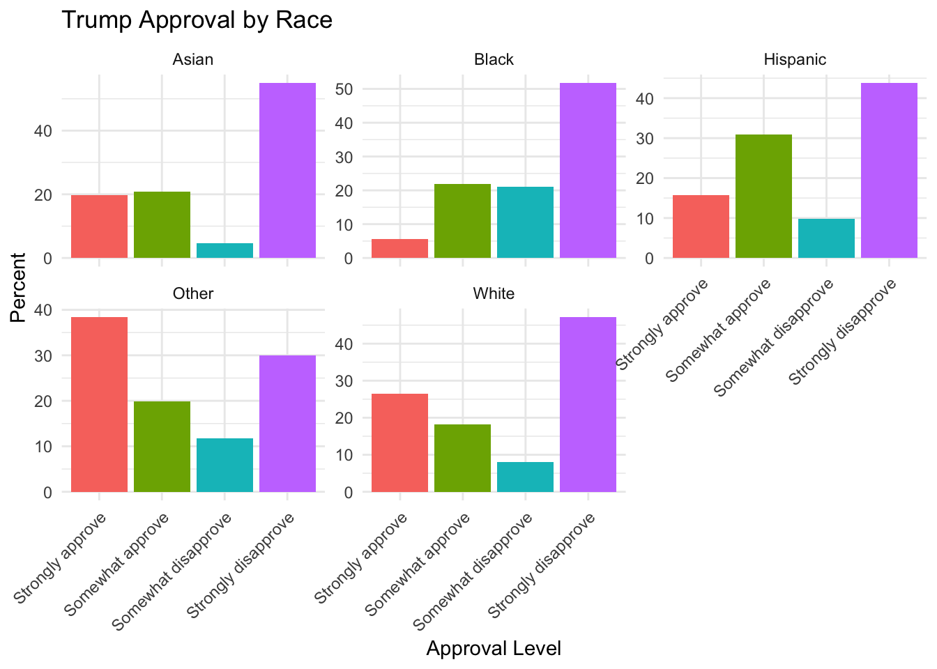
pewmethods::get_totals("trump_approval", sm.out, wt="weight", by="race", na.rm=T)
#>        trump_approval weight_name     White  Hispanic
#> 1    Strongly approve      weight 26.543060 15.685443
#> 2    Somewhat approve      weight 18.162720 30.819294
#> 3 Somewhat disapprove      weight  8.109798  9.766586
#> 4 Strongly disapprove      weight 47.184421 43.728677
#>       Black     Asian    Other
#> 1  5.546739 19.634503 38.40852
#> 2 21.827358 20.884765 19.92100
#> 3 20.956283  4.609946 11.67791
#> 4 51.669620 54.870786 29.99256
And now we get a nice crosstab of trump support by each racial demographic.
Where you go from here is really up to you, and we will see examples as we go along. We want to take these results and crosstabs and work them into stories and visualizations.
I will say that one nice thing about the get_totals package is that it produces a tibble which is the tidyverse style of data. This makes it easy to take the output and reshape it into something that could go into ggplot, for example:
pewmethods::get_totals("trump_approval", sm.out, wt="weight", by="race", na.rm=T) |>
  pivot_longer(cols=White:Other,
               names_to = "race", values_to = "percent") |>
ggplot(aes(x = trump_approval, y = percent, fill = trump_approval)) +
  geom_col() +
  facet_wrap(~race, scales = "free_y") +
  labs(
    title = "Trump Approval by Race",
    x = "Approval Level",
    y = "Percent"
  ) +
  theme_minimal() +
  theme(
    legend.position = "none",
    axis.text.x = element_text(angle = 45, hjust = 1)
  )