1 Introduction

1.1 Public Opinion Polling is Inescapable

This is a class on public opinion polling. When we think of that term a lot of us immediately think about election polling.

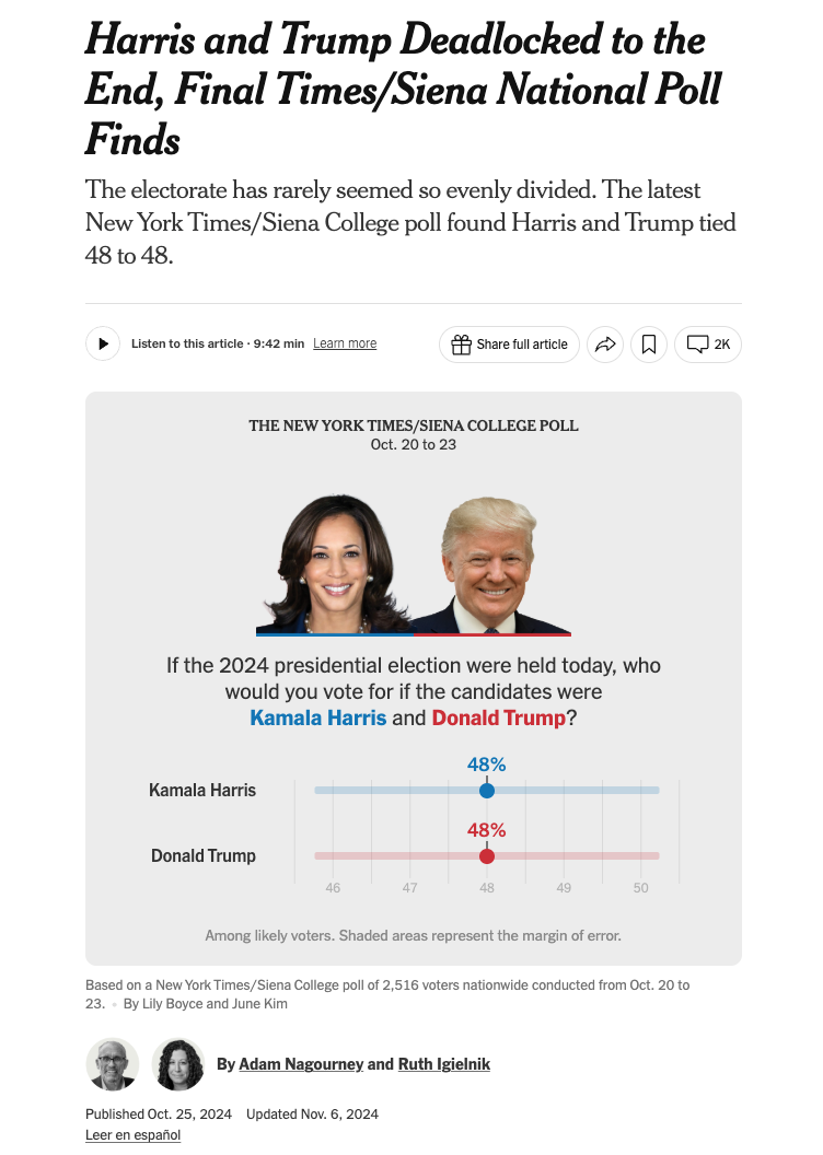
Polling around elections play an out-sized role in what the public thinks about when we think about “polling”. So much so that it hides the absolutely crucial role that polls play in our lives. I would contend that we focus so much on election polls because (a) the information stemming from them is clearly branded as coming from a survey; (b) we feel really strongly about what they are telling us; (c) we get to see the real answer (the election result).

But think about this:

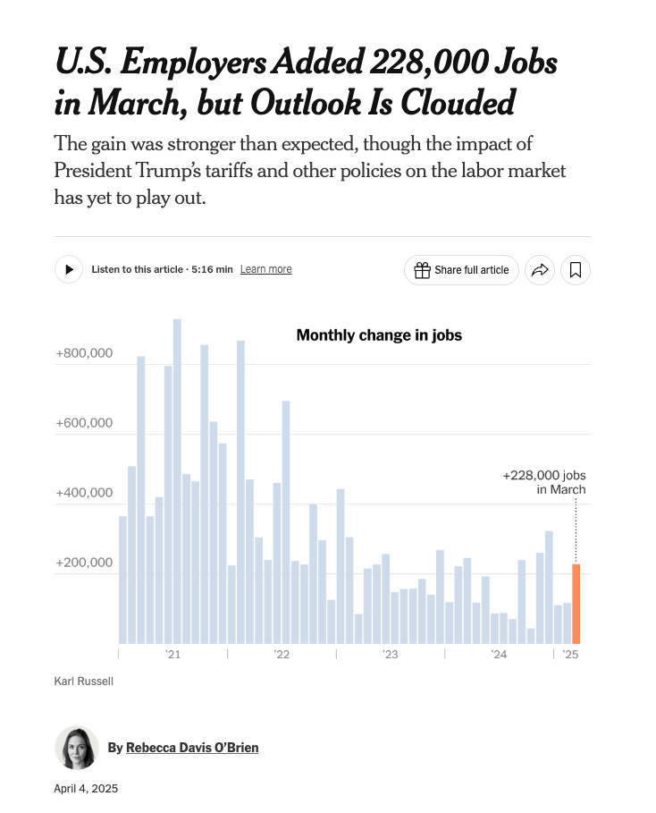
Here is a NYT article from April on the job report. It says that in March 2025 the US added 228 thousand jobs and the unemployment rate rose from 4.1% to 4.2%.

How did the Labor Department determine these numbers? Is there some databank out there of every job in the United States, such that we could see that there are 228 thousand new entries? Is there similarly a database of every American and what job they are working so that we know what percent are currently unemployed? No! Neither of these things exist.

The job report actually comes from two surveys, one of businesses and government agencies and another of households. Together they use these surveys – where statisticians speak to a small fraction of the businesses and households in the United States – to determine the number of jobs available and the number of people who are “unemployed”. As a side note, people generally misunderstand what it means to be unemployed: to be unemployed you must not have a job (duh), be available for work, and have to have actively looked for work within the past four weeks. If you don’t meet these criteria (say if you have a disability that prevents you from working, or if you have given up from looking for a job) then you are not counted in the denominator.

After an election we spill barells of ink determining if the polls were accurate. So is the unemployment rate accurate? We have no idea. Elections are special because we are polling for an event that really happens that we get real numbers from. There is no “Unemployment Election” where we all have to show up and register if we are working or not, so there is no true event that benchmarks the unemployment rate. We don’t think about this being a poll that has error because we never get to see the error.

Or how about another example, if I just Google something innocuous like:

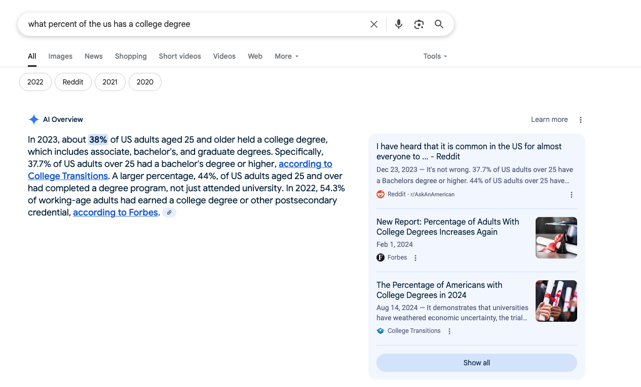
I can find out that 38% of the US has a college degree.

But again, where could this number possibly come from? Well there is the Census, which is not a survey, and actually tries to count every person. But the Census doesn’t ask about education, it just asks sex, age, race, and household ownership.

As such any statistic about the demographic composition of the US (or states, or cities) that isn’t one of those things necessarily comes from a survey.

That’s not to say that there are no other sources than surveys. There exist administrative records for many things that allow us to avoid the potential sources of error that come from surveys. (Though these things introduce different potential sources of error.)

So, for example, we can get dashboards like these:

When distributing COVID vaccines the Philly department of health kept track of the age, gender, and race of those receiving them, so we can get a relatively accurate sense of who was receiving the vaccine.

But what if I asked: what percentage of White Philadelphians received the vaccine. Well… what percent of Philadelphians are White? We are back to the same problem of having to use a survey to get this answer.

Surveys are ultimately an inescapable necessity of understanding the world that we live in. There are things for which we keep administrative records, and for very rare things we count everyone (the Census), and we have one special thing where everybody records their preference on the same day (elections). But for everything else the only way to actually understand the nature of mass public is through a survey.

1.2 What makes a survey a survey?

What formally defines a survey? According to Groves:

A survey is a systematic method for gathering information from a sample of entities for the purposes of constructing a quantitative description of the attributes of the larger population of which the entities are members.

A couple of key terms here. Surveys are systematic because we are applying a clearly defined methodology to the process. They are quantitative because we are measuring attributes systematically. And finally the key feature is that we are using a sample of data to understand the attributes of a full population.

This latter thing – understanding the broader population from a sample of data – is the fundamental hallmark of a survey. Instances where we try to capture the population by capturing every member of the population (a census) do not count as surveys.

Censuses have been around for thousands of years. In the Bible, for example, we have in Numbers:

Take ye the sum of all the congregation of the children of Israel, after their families, by the house of their fathers, with the number of their names, every male by their polls; From twenty years old and upward, all that are able to go forth to war in Israel: thou and Aaron shall number them by their armies.

Or in Luke:

In those days a decree went out from Caesar Augustus that all the world should be registered.

So this idea is old.

But the idea that we can shortcut this process by only looking at a small number of people out of the whole is a relatively new idea. It’s relatively new because the mathematical tools needed to understand why this works are relatively new. Statistics as a branch of mathematics only solidified in the 20th century.

So shooting ahead, pollsters started to become prominent in the 1920s and 1930s. These early survey researchers were trying to measure many things, including information for businesses. But much like today their most public product was the prediction of elections.

The earliest survey that tried to predict elections in a systematic way was the Literary Digest poll. They knew they could not do a Census of all voters, so their methodology was to sample as many people as possible. If data is good, more data is better, so they thought (they were wrong). To get their numbers they voraciously bought up lists of individuals: telephone directories, car registration records, rosters of clubs and associations, occupational records, etc. They tried to get as many addresses for as many voters as possible and mailed out as many as possible surveys. In 1930 they mailed 20 million voters a survey, and had over 400 clerks tabulating the replies.

Early on, this big-data poll had a run of success, correctly predicting the 1924, 1928, and 1932 elections. Indeed, the average error for thie predictions was 3%. That’s very good!

In 1936 they sent out 10 million postcards and had 2.4 million responses. After tabulation they published that Republican Alf Landon would prevail with 55% of the vote. And we all remember how President Alf led us confidently through the darkness of WWII, and his face shines brightly from the slopes of Mt. Rushmore as one of our greatest presidents.

So no, Alf Landon did not win 55% of the vote. Indeed, he lost in a landslide with FDR winning 61% of the population vote and all but 8 electoral college votes. This was a polling disaster, and largely bankrupted Literary Digest.

What went wrong? We will formalize these things in the coming weeks, but the short answer is that the people who returned their ballots were the wrong people. The lists that were available to Literary Digest were biased towards Republicans, particularly automobile owners and those who owned a telephone (and would therefore be in the phone book). In the parlance of survey research this is a sample frame problem: the list of people they had to reach out to were not representative of American voters.

But that was not the only problem with the Literary Digest poll. Recall that 10 million postcards were sent out but only 2.4 million were returned. Among the people who received the postcard, people who supported Landon were more likely to return their postcard compared to people who supported Roosevelt. This is a problem that we will come to learn as non-response bias – the people who decide to respond to the survey conditional on being contacted are a non-representative group of people. This second problem, unfortunately, was not well understood at the time, and the statistical literacy needed to untangle it was not well understood.

As such, the “solution” to the 1936 debacle was focused on the “sampling frame” part of the problem. To rush in and fix these problems were a younger crop of survey researchers who employed “quota sampling”. Foremost amongst them was George Gallup - he’s famous! You know him!

The notion of “quota” sampling directly addressed the sample frame problem from above. Gallup, and pollsters like him, set targets for categories of people to talk to that were proportional to the size of those groups in the population. Gallup split the population into a number of categories – for example “Industrial homes of skilled mechanics, mill operators, or petty trades people (no servants)” – and included in his sample the same proportion of those people as are in the greater population.

The systematic nature of this poll was different from the Literary Digest poll, but also of importance is that this dramatically reduced the number of people surveyed. Where Literary Digest had a “more data better” approach, Gallup had a “small and better data” approach. This was the major critique of the poll at the time: how could a poll work if you didn’t know anyone who was polled? But the initial predictive power of this survey won over the critics. Gallup successfully predicted the 1936 election which Literary Digest got wrong, as well as the 1940 and 1944 elections.

The most important improvement being made here was sampling – and we will have a lot more to say about that. But also during this period was improvements in the systematic nature of polls. In previous periods of polling you might have a list of things that you want to know and simply send out people to gather that information: go figure out a bunch of people’s age, income, gender, and who they are voting for. Survey practitioners started to realize, however, that the way that these questions were asked could potentially lead to different answers. Part of the process of professionalizing the operation was to start to produce standardized questions that would be read verbatim to each respondent, and having more strenuous training of interviewers to ensure standardization.

Come the 1948 election this young group of pollsters – Gallup and Roper and the rest – had become stars, and were getting cocky. The pollsters, using their quota sampling methodology, predicted a strong win for Republican Thomas Dewey. Gallup said before the election “next Tuesday the whole world will be able to see down to the last percentage point how good we are.” And, indeed, he was tragically correct. Dewey’s Presidency, as we all know, ended in infamy, shame, and the complete destruction of Toledo, Ohio.

OK, no. Truman won the election relatively handily, thereby embarrassing a new crop of pollsters.

What went wrong? In this case it was interviewer freedom which led to the errors. Quotas were set by the company, but interviewers in the field had wide latitude to go out and get who they could to fill these quotas. This led to an under-sampling of the very poor and the very rich. Said one pollster the problem was “the difficulties interviewers encounter in questioning the unshaven and sweaty”.

We have arrived at the critical juncture where the pollsters figured it out, and the method that allowed them to figure it out is random sampling. The Gallup method relied on carefully selecting respondents to match certain population proportions. That led to the problem of interviewer bias in who they selected in each of the categories.

As it turns out there is a much more direct way to do this, which is random sampling the population.

Let me briefly show you how this works. We are going to generate a population from which we are going to take a sample:

library(tidyverse)
library(MASS)
set.seed(123)
n <- 100000
cor_matrix <- matrix(c(
  1.00,  0.20,  0.20, -0.10,  0.40,  # male
  0.20,  1.00,  0.30,  0.25,  0.50,  # white
  0.20,  0.30,  1.00,  0.35,  0.45,  # rich
 -0.10,  0.25,  0.35,  1.00, -0.30,  # college
  0.40,  0.50,  0.45, -0.30,  1.00   # vote.republican
), nrow = 5, byrow = TRUE)

# Simulate latent traits
latent <- mvrnorm(n = n, mu = rep(0, 5), Sigma = cor_matrix)

# Thresholds to get realistic marginal distributions:
# ~50% male, ~60% white, ~25% rich, ~55% college, ~40% vote.republican
male             <- latent[, 1] > 0
white            <- latent[, 2] > -0.25
rich             <- latent[, 3] > 0.67
college          <- latent[, 4] > -0.13
vote.republican  <- latent[, 5] > 0

# Combine into a data frame
pop <- data.frame(
  male = male,
  white = white,
  rich = rich,
  college = college,
  vote.republican = vote.republican
)

pop |> 
  summarise(across(everything(), mean))
#>      male   white    rich college vote.republican
#> 1 0.50076 0.59858 0.25107 0.55117         0.50135

This population is 50% male, 60% white, 25% rich, 55% college educated, and voted 50% Republican. Even in our simulations our elections are tied.

Now, obviously, if we sample every single member of this population, we will get the exact same distribution for these variables:

samp <- pop[sample(1:nrow(pop), nrow(pop), replace=F),]

samp|> 
  summarise(across(everything(), mean))
#>      male   white    rich college vote.republican
#> 1 0.50076 0.59858 0.25107 0.55117         0.50135

The critical think about random sampling is that we can take a much smaller sample, and as long as that sample is random, the distribution of these variables will be identical to the population in expectation.

So if we take a sample that is half the size of the population:

samp <- pop[sample(1:nrow(pop), 50000, replace=F),]
samp |> 
  summarise(across(everything(), mean))
#>      male   white    rich college vote.republican
#> 1 0.50008 0.59862 0.25114  0.5518         0.50074

We get approximately the same distribution.

Or a sample of 1000 people:

samp <- pop[sample(1:nrow(pop), 1000, replace=F),]
samp |> 
  summarise(across(everything(), mean))
#>    male white  rich college vote.republican
#> 1 0.505 0.591 0.264    0.53           0.525

Approximately right.

Or 100 people:

samp <- pop[sample(1:nrow(pop), 100, replace=F),]
samp |> 
  summarise(across(everything(), mean))
#>   male white rich college vote.republican
#> 1 0.52  0.57 0.28    0.63            0.56

Further off, but still approximately right.

We will learn a lot more about this in a few weeks when we talk about sampling. What’s critical here is that random sampling allows us to make unbiased inferences about populations from small samples of data.

Further, according to traditional statistical theory the size of the population doesn’t matter at all in this process. A survey of 1000 people in Canada (40 million people) has the same predictive power as a survey of 1000 people in the United States (336 million people) which has the same predictive power of a survey of 1000 people in China (1.4 billion people).

The best analogy for why this works is making a pot of soup. If you want to know whether your soup has enough salt in it, do you need to eat an entire bowl? No, conditional on stirring it well (that’s the random sampling) you just need a spoonful to judge the seasoning level. And it doesn’t matter if your pot is big or small, we use the same spoonful to understand the saltiness.

We can also use this population to help us understand what went wrong in things like the Gallup or Literary Digest polls.

Say that we sample 1000 people, but better educated people are slightly more likely to be interviewed. We can simulate this with a variable that is equal to 15% if someone does not have a college degree and 20% if someone does have a college degree:

pop |> 
  mutate(interview.prob = if_else(college==T, .20, .15)) -> pop

And now when we sample, we will sample according to those probabilities:

samp <- pop[sample(1:nrow(pop), 1000, replace=F, prob=pop$interview.prob),]
samp |> 
  summarise(across(everything(), mean))
#>   male white  rich college vote.republican interview.prob
#> 1  0.5 0.597 0.266   0.625           0.483        0.18125

Of course, when people who are more likely to have a college degree have a higher probability of being in the sample we estimate more people have a college degree than in the population. But because all of these variables are correlated, making such an error also screws up all the other probabilities. Critically, we have now under-estimated the Republican vote share (by about 4 percentage points) because college educated people are more likely to vote Democratic.