5 Sampling I
5.1 Introduction
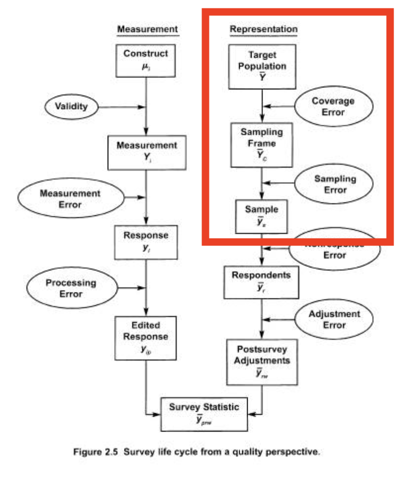
We now want to move to the left side of the “error tree” from the survey research overview chapter.
We are going to start with a small review of target populations, sampling frames, and coverage error. We will then move on to the main topic, which is sampling and sampling error. This is where we will get the most “stats heavy” in this class. We will look at the statistical properties of “simple random samples” (SRS) first, before moving on to the complications of finite populations, cluster sampling, and stratified sampling. We will wrap up the two weeks with a more in-depth look at the Literary Digest poll of the 1930s, which serves as a cautionary tale.
5.2 Populations, Frames, and Coverage Errror
This section will talk more about moving from a target population to a sampling frame to a sample, and the errors that can occur through that process.
The actual units that we wish to sample in this framework are called “elements”. This is a little more complicated then “who are we talking to”. We could be interested in sampling US Adults, or registered voters, but we could also be interested in sampling households or businesses, and we speak to a person within those elements as a sort-of representative. Elements have to be observable, and are defined within a certain time frame. This latter thing is important as people can move in and out of a population. Consider “registered voters”. This is a common population, but one that is constantly shifting.
The universe of all the elements that we wish to study is the “population”. Again, for all US Adults this would be…. all adults in the US during the period we are studying. Election polls are special because the population is the people who will vote in the future (we will discuss this a lot more!).
The “sampling frame” is the real list or process that tries to contain every element in the population. This is not the sample itself, but an enumeration of all of the population. I say here list or process because this is only sometimes and actual list. The voter file, for example, is a real list of the registered voters in the United States (though, with over and undercoverage, as described below). However, if we are doing an online survey we almost certainly do not have an actual list of all US Adults (for example), instead we believe our process gives us access to all US Adults. Similarly a random digit dial survey is a process that gives us access to all US Adults with a telephone.
There is a lot of complicated stuff in the Groves chapter that may or may not every apply to you. To be honest a lot of the issues in surveys discussed comes from the period of time where a lot of surveying was happening by calling and mailing a house when your target population are individuals.
The fundamental thing that you need to know is this: your sampling frame ideally gives every element in the population a known and non-zero probability of being selected.
In the ideal case you have a sampling frame which truly lists every member of the population. In this case each person is listed once and only once, and as such, each person has a non-zero and equal probability of being selected into your sample.
5.2.1 Under Coverage
The most extreme case of breaking this tenet is “under-coverage” which is the case when there are elements of the population that are not in your sampling frame at all. In this case their probability of being selected into the sample is now zero.
In traditional telephone surveys under-coverage obviously comes from people who do not have a phone number. In an RBS survey under-coverage can come from bad maintenance of voter file lists, where recent registrants have not been added to the voter file when we make our sampling frame. For online surveys under-coverage exists because the process which represents the sampling frame doesn’t actually give a non-zero probability to every US Adult (for example) – some people aren’t online and have a zero probability of being in the survey.
Just because there is under-coverage, however, doesn’t mean that you will have coverage error in your survey.
Coverage error survey can (theoretically!) be calculated through the formula:
\[ Cov.Error = \frac{U}{N}(\bar{Y_c} - \bar{Y_u}) \]
Where \(U\) is the total number of uncovered people, \(N\) is the total number of people in the population, \(\bar{Y_c}\) is the value for the variable we are studying for the people who are in the sampling frame, and \(\bar{Y_u}\) is the value of the variable for the people who are not in the sampling frame.
So let’s say we are studying a population of 1000 people via RDD and 100 people do not have a phone. The people who do have a phone have a presidential approval of \(40%\) and the people who do not have a phone have a presidential approval rating of \(50%\). This means that coverage error would be:
(100/1000)*(.4 -.5)
#> [1] -0.01
Negative 1 percentage point.
What should be clear from this equation is that both terms can easily go to zero and wipe this whole thing out.
If the proportion of uncovered people is small (\(U\) is small relative to \(N\)) it doesn’t much matter what \((\bar{Y_c} - \bar{Y_u})\) is.
Similarly if the difference in the opinions of those covered and those not covered is small \((\bar{Y_c} - \bar{Y_u}) \rightarrow 0\), then it doesn’t really matter what proportion of people are uncovered.
To put a finer point on this: we only care about under-coverage if the opinions of those not covered are systematically different than those who are covered.
The other consideration with under-coverage is if it is systematic enough to actually change the definition of the population in order to match what is possible with the sampling frame. This is less stupid than it sounds. Groves gives the example of starting out with a research goal of assessing the learning goals of all students in the US. Public school students are possible to put on a sampling frame (all public schools can be listed, and then the students in those schools can be listed). But private school kids are more difficult. It is not unreasonable in that case to re-define the population of interest to be “students in US public schools”.
5.2.2 Inelegible units
The opposite problem occurs when there are eleements in our sampling frame who should not be there. Similar to the above, we only really care about this if these people have systematically different opinions then the eleigible people, and would therefore bias the results.
However, the nice thing about having inelegible units is that you actually get to talk to these people if you sample them. If we are studying registered voters and we call someone who is not a registered voter, we can simply ask if they are an ineligible voter and exclude them from the study! So this is generally a much less serious problem.
Where I think this is more of a problem is in pre-election studies, where the target population is the people who will vote in the future. Those who will not vote are technically “ineligible units”. But we are now trying to predict future ineligibility, something that a respondent may not even know. This is a really hard problem, and represents a level of potential error that is really unique to election polling.
5.2.3 Complicated non-zero probabilities
In some surveys there can be some complicated probabilities associated with the sampling frame that need to be adjusted for.
I don’t want to get too deep into this, because it is unlikely that you will be designing a telephone survey in 1997, but I think it’s worth discussing this sort of thing because it can broadly apply to other types of sampling frame construction (and will relate to stratified sampling below.)
When I introduced the sampling frame issue I said that elements must have a “known and non zero probability” of selection.
We have dealth with the “non-zero” part of this, but the more complicated thing is having a known probability.
The clearest example of this is when the elements are people but you are sampling households.
Let’s say you have 10000 houses in your sampling frame, which represents an unknown number of actual people (the elements), and you wish to sample 1000 people.
If you call (or mail!) a household with 2 people in it and one person is randomly selected to fill out the survey, then that person had a \(\frac{1}{1000}*\frac{1}{2} = \frac{1}{2000}\) probability of being selected into the survey.
Consider a second household with 5 people in it, one of whom is similarly randomly selected to fill in the survey. That person had a \(\frac{1}{1000}*\frac{1}{5} = \frac{1}{5000}\) probability of being selected into the survey.
People in smaller houses therefore have a higher a priori probability of being included in the survey then people in larger houses. If people who live in houses with more people have systematically different opinions than people who live in houses with less people, then not correcting for this will give you a biased estimate.
Thankfully this is easy to correct for if you simply know the number of people that live in each house. The person from a house with more people will be given a higher selection weight, which will then be multiplied by any other weight that is derived. In that way we correct for unequal probability of selection into the sample.
5.3 Sampling Error for Simple Random Samples
When you read a poll release on a news website it will say something like “These results accurate to plus or minus 2.1 percentage points, 19 times out of 20”, or “The margin of error of this poll is plus or minus 2.1 percentage points.”
At the conclusion of this section you will understand exactly how these numbers are arrived at.
Actually: I can just tell you exactly how these numbers are arrived at.
The margin of error of a poll is determined by:
\[ MOE = 1.96 * \sqrt{\frac{.25}{n}} \]
Where \(n\) is the number of people in a poll. If there are 2177 people in a poll then:
1.96*sqrt(.25/2177)
#> [1] 0.02100375
The margin of error is plus or minus 2.1 percentage points.
So more accurately, you will learn why the above formula is how we arrive at the margin of error, and theoretically what we mean when we list that margin of error.
5.3.1 Start with a coin
What do we mean when we say that a coin comes up heads 50% of the time?
If we flip a fair coin 10 times we don’t always get exactly 5 heads and 5 tails:
coin <- c(0,1)

sum(sample(coin, 10, replace=T))/10
#> [1] 0.4
sum(sample(coin, 10, replace=T))/10
#> [1] 0.2
sum(sample(coin, 10, replace=T))/10
#> [1] 0.7
sum(sample(coin, 10, replace=T))/10
#> [1] 0.6
sum(sample(coin, 10, replace=T))/10
#> [1] 0.6
We get something a little bit different everytime.
What we want to do is to understand the regular properties of this “little bit different every time”.
Thinking in terms of a coin is particularly helpful for survey research because many of the things that we are looking at in a survey are proportions.
When we looked at the coin above we made heads=1 and tails=0, and in each trial we looked at the proportion of 1s. Coins are a particular instance of a broader things we call Bernoulli Random Variables. We are not going to get into what a “random variable” is in this class, but it’s enough to say right now that it’s a way of summarizing data generating processes (like flipping a coin). Other random variables include the “Normal” random variable (a bell curve) which generates things like height.
A fair coin is a Bernoulli random variable where the probability of success (which we denote as \(\pi\)) is .5 or 50%. But we can think of other phenomenon in the same framework, while changing the probability of “success”. Note that “success” here is just the technical term given to one of the two outcomes, the thing we are denoting “success” doesn’t have to be a normatively good thing or anything.
In the 2022 Pennsylvania Senate election (which was a recent election when I first wrote these notes) John Fetterman won 2,751,012 votes and Mehmet Oz won 2,487,260 votes, which means that Fetterman won 52.5% of the vote.
If we think about sampling Pennsylvania voters before the election (ignoring people who vote for third parties and don’t vote, for simplicity right now) we can think about each person we sample as a coin that comes up Fetterman 52.5% of the time. In other words, a Bernoulli Random Variable where the probability of success \(\pi\) is .52.
#The sample command lets us assign probabilities to each instance in coin
sample(coin, 10, prob = c(.52,.48), replace=T)
#>  [1] 0 1 0 0 0 1 0 1 1 1
sample(coin, 10, prob = c(.52,.48), replace=T)
#>  [1] 1 1 1 1 0 0 0 1 1 1
sample(coin, 10, prob = c(.52,.48), replace=T)
#>  [1] 0 1 0 0 0 1 0 0 1 1
sample(coin, 10, prob = c(.52,.48), replace=T)
#>  [1] 1 1 1 1 0 1 1 1 0 1
That’s a helpful example because we know the true answer, but we could also think about sampling people about whether they approve of Donald Trump, or not. In that case that’s like a coin/Bernoulli RV that comes up “Approve” 43% of the time (or whatever Trump’s “true” approval rating is.)
#The sample command lets us assign probabilities to each instance in coin
sample(coin, 10, prob = c(.43,.57), replace=T)
#>  [1] 1 0 0 1 1 0 1 1 1 0
sample(coin, 10, prob = c(.43,.57), replace=T)
#>  [1] 0 0 1 0 1 0 1 1 1 0
sample(coin, 10, prob = c(.43,.57), replace=T)
#>  [1] 1 1 0 0 0 1 1 0 0 1
sample(coin, 10, prob = c(.43,.57), replace=T)
#>  [1] 0 1 0 1 1 0 0 0 0 1
So how we want to proceed is to think about the properties of taking large samples of “coins” (really Bernoulli Random Variables), when those coins can have any probability of coming up heads between 0 and 1. This serves as a helpful “model” for survey response as many of the things we are studying are proportions. (I will discuss how we generalize this to non-proportions at the end.)
5.3.2 Law of Large Numbers and Central Limit Theorem
We want to understand if there is any regularity to sampling. Can I predict, before I take a sample of 5000 people, how much variance I can expect compared to other samples of 5000 people? How is that different than if I sample 100 people? Or 1 million people?
Let’s say I am sampling Pennsylvanian voters in November 2022, who had a true probability of supporting Fetterman over Oz of .525. That is, if we think of each PA voters as coins that have one side “Fetterman” and one side “Oz” the probability of flipping a Fetterman is .525.
To be more statsy: we can think about each voter being a Bernoulli random variable with a probability of success of .525. I’m going to create a sample of 10,000 voters drawn from this Bernoulli Random. I’m going to sample all 10,000 at once but we can interrogate the first 10 voters as a sample of 10, the first 50 as a sample of 50, the first 100 as a sample of 100 etc. The rbinom() command is working just like our sample command above, but is purpose fit for this task and therefore works a bit more efficiently. We are similarly telling it to “flip” 10000 coins where the probability of heads (Fetterman) is 52.5%.
set.seed(19104)
samp <- rbinom(10000,1,.525)
head(samp, 50)
#>  [1] 1 1 0 1 0 1 0 1 1 0 1 1 1 0 1 0 0 0 1 1 1 1 1 0 1 0 0 0
#> [29] 0 1 0 1 1 0 0 0 0 1 1 0 1 1 1 0 1 1 1 0 1 0
We know that the “truth” that we are sampling from is a success rate of .525. We want to know how relatively close an estimate made at different sample sizes is. So for each “sample size” from 1 to 10,000 I’m going to calculate the proportion of people supporting Fetterman. We will start by looking at the first 1000 samples.
#The cumsum() function adds up every value that occurs previous in a vector

cumulative <- cumsum(samp)

#Divide by the position to get the average at each value

relative.error <- cumulative/1:length(samp)

head(samp)
#> [1] 1 1 0 1 0 1
head(cumulative)
#> [1] 1 2 2 3 3 4
head(relative.error)
#> [1] 1.0000000 1.0000000 0.6666667 0.7500000 0.6000000
#> [6] 0.6666667


plot(1:10000,relative.error, xlab="Sample Size",ylab="Fetterman Percent", type="l",
     ylim=c(0.3,0.7), xlim=c(0,1000))
abline(h=.525, lty=2, col="firebrick")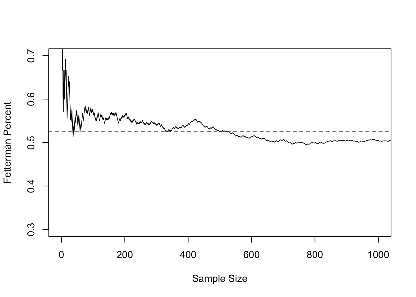
This line represents the sample mean at each sample size, from 1 up to 1000.
At sample size of 1 we are guaranteed to be quite far off from the truth, because the average at that point must be 0 or 1. But relatively quickly the 0’s and 1’s start to cancel out and by a sample of 50 we are down near the truth. From 200 to 1000 we continue to jump around, approximately around the true value of .525, however.
Let’s extend to look at the full 10,000:
plot(1:10000,relative.error, xlab="Sample Size",ylab="Fetterman Percent", type="l",
     ylim=c(0.3,0.7))
abline(h=.525, lty=2, col="firebrick")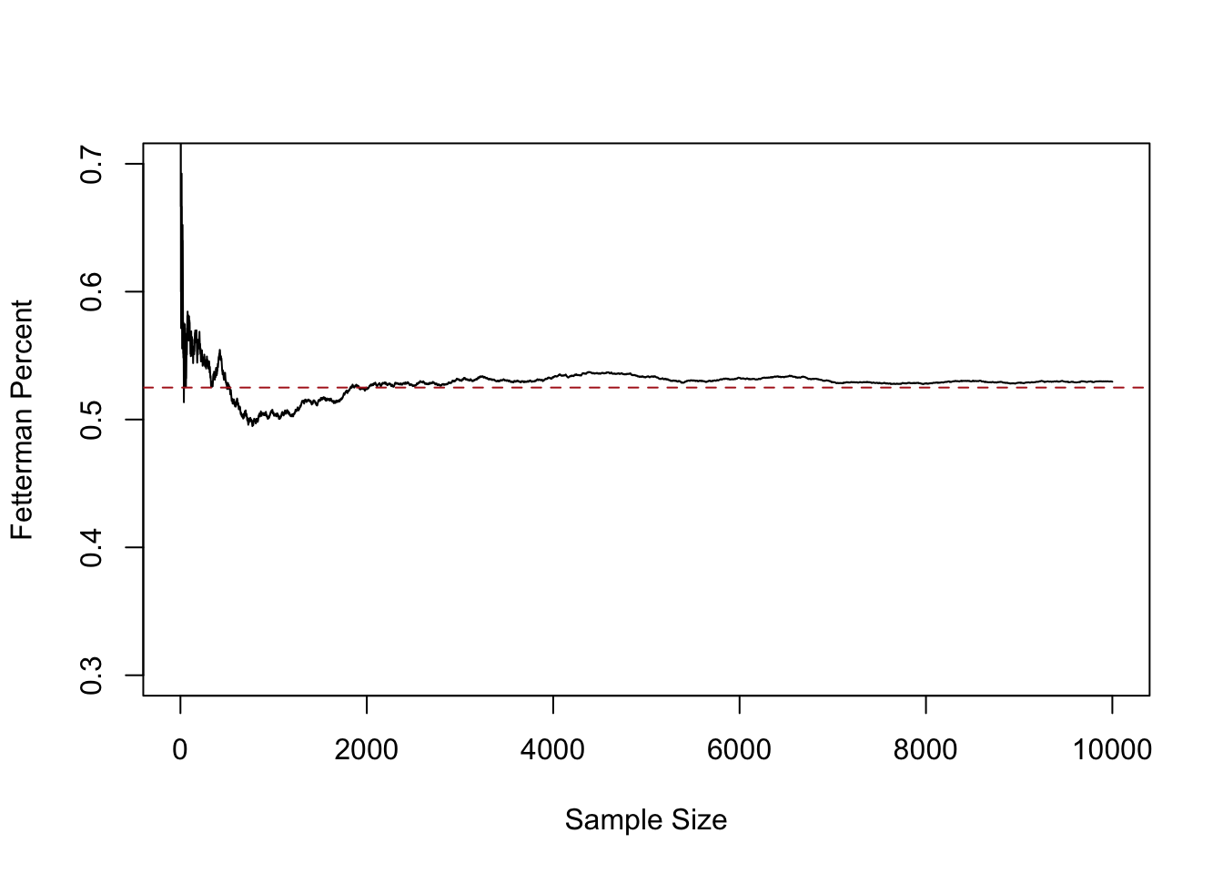
Here we see that after a sample size of about 2000 we get pretty close to the truth and stay relatively close to it.
This fact: that as the sample size increases the mean of the sample approaches the true population mean, is what is known as the Law of Large Numbers. To state it mathematically:
\[ \bar{X_n} = \frac{1}{n} \sum_{i=1}^n X_i \rightarrow E[X] \]
There are a couple of new things in here that we should slow down to take note of. The \(X\) with no subscript is the random variable we are sampling from. In the running example this is a Bernoulli RV with probability of success of .525. \(n\) represents the number of observations that we currently have. \(n\) will (I think, probably) always represent this. To the point where people will say “What’s the \(n\) of your study?”. \(X_i\) represents our sample from the random variable \(X\), and \(i\) is the index number for each observation. So for example: what are \(X_i\) 1 through 10:
samp[1:10]
#>  [1] 1 1 0 1 0 1 0 1 1 0
\(\bar{X}_n\) is the average across all observations. We usually put a bar over things that are averages.
\(E[]\) is the expected value operator. This is sort of like probabilities version of a “mean”, but is a theoretical concept that denotes the long-run average outcome of a random variable.
Overall, this statement says that the sample average (add up all the X’s and divide by the sample size) approaches the original Random Variable’s expected value as the number of observations increases.
As we will see, this is true of all random variables, not just a Bernoulli.
So the first principle of sampling:
- The larger a sample the more likely our sample mean equals the expected value of the random variable we are sampling from (LLN).
That’s helpful, but we still don’t have a good sense of being able to answer a question like: If I run a sample of 500 people, how much can I expect to miss the truth by?
To help us understand this, let’s dramatically ramp up what we are doing here. Right now we have one “run” of a sample of 1,2,3,4,…. all the way up to 10,000. I’m going to add 999 more samples of 10,000 people. I’m also going to highlight the original run in magenta.
set.seed(19104)
binomial.sample <- matrix(NA, nrow=10000, ncol=1000)

for(i in 1:1000){
  binomial.sample[,i]<- cumsum(rbinom(10000,1,.525))/1:10000
}

plot(1:10000,binomial.sample[,1], xlab="Sample Size",ylab="Fetterman Percent", type="n",
     ylim=c(0.3,0.7))
for(i in 1:1000){
  points(1:10000,binomial.sample[,i], type="l", col="gray60")
}
abline(h=.525, lty=2, col="firebrick")
points(1:10000, binomial.sample[,1], col="magenta", type="l")
abline(v=c(100,500,1000,5000,10000), lty=2, col="darkblue")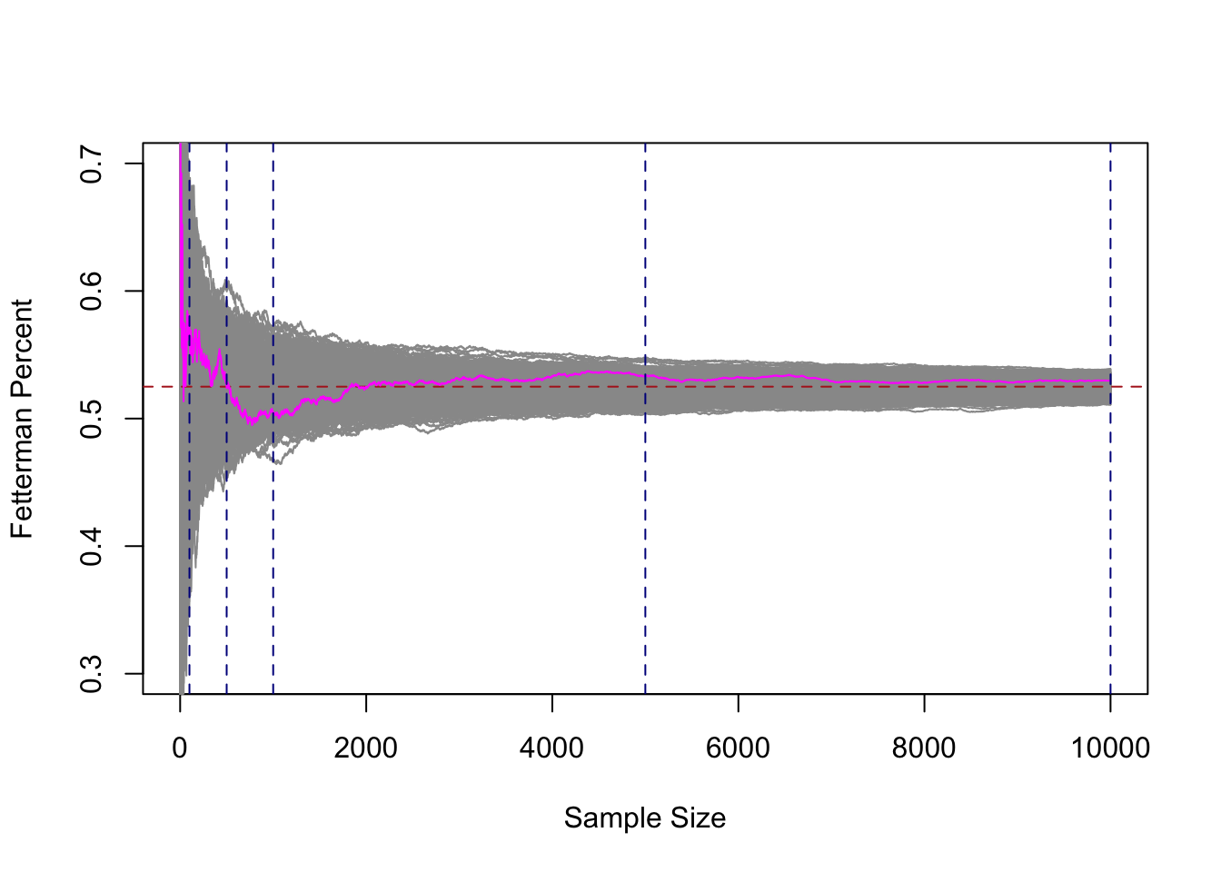
Each of these gray 1000 lines represents a cumulative sample of 1 all the way up to 10,000 units. If we look at any vertical cross-section of these lines, that represents 1000 means from 1000 surveys at that \(n\). Just as our original magenta line at position, say 50, represents the mean of this sample when n=50. In other words: any cross-section of this graph tells us what it’s like to have 1000 surveys of 500 people, or 1000 surveys of 503 people, or 1000 surveys of 8000 people….
There are a couple of very important things about this graph so we can take some time to consider it.
If we take any given cross section of the data (i’ve highlight 100,500,1000, and 10,000, but there is nothing special about those numbers), there are some surveys that are well below the target, and some surveys that are well above the target. However, we also see that if we consider all 1000 surveys together they are centered on the true value of .525. The number of surveys that miss high are perfectly balanced by the number of surveys that miss low.
Indeed, if we look at the “average of the averages”:
means <- rep(NA,1000)

for(i in 1:1000){
means[i] <- mean(binomial.sample[,i])
}

plot(1:1000, means, pch=16,
     ylim=c(0.3,0.7), xlab="Average of Averages", ylab="Sample Size")
abline(h=.525, col="firebrick", lty=2)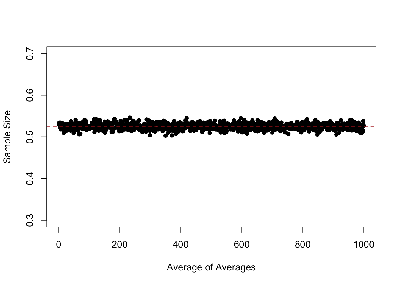
At every level of \(n\) they are approximately equal to the expected value of the distribution that we are sampling from. So while lines are missing by a whole lot in small sample sizes, the average of a large number of samples still equals the expected value of the distribution that we care about.
The law of large numbers tells us that as sample size increases the estimate we form is more likely to converge on the expected value of the distribution that we care about.
What we’ve uncovered here is something different, and even more helpful. For any sample size, the expected value of the sample mean is the expected value of the distribution that we are sampling from.
If I am doing a survey of 10 people I do not expect that my guess will be very close to the truth. However if before I take my sample you ask me what I expect will happen, I will tell you that my best guess is that the mean of my sample will be equal to the expected value of the random variable I am sampling. That’s true if I have a sample of 10, 100, 1000, or a million. My answer to that question never changes.
So far we have:
- The larger a sample the more likely our sample mean equals the expected value of the random variable we are sampling from (LLN).
- For any sample size, the expected value of the sample mean is the expected value of the random variable we are sampling from.
The third principle of sampling we can visually see: the distribution of means at any given sample size decreases as the sample size increases. At very low n our guesses (while centered in the right place), are all over the place. Way too high, Way too low. Ranging from .7 all the way to .3. As the sample size increases the LLN kicks in and all the samples get close to the truth.
But is the “amount they miss on average” something that is measurable?
To understand that, let’s look more closely at the 4 cross-sections I made in the graph about at benchmark sample sizes: 100,500,1000,5000, and 10,000. What we are going to do now is look at the density of the samples at all of these points. Think about taking a knife and making a cross-section at each of these blue lines, we are going to do that and plot what that particular cross section looks like.
par(mfrow=c(2,3))
plot(density(binomial.sample[100,]), main="Sampling Distribution at n=100", xlim=c(0.3,0.7))
abline(v=.525, col="firebrick", lty=2)
plot(density(binomial.sample[500,]), main="Sampling Distribution at n=500", xlim=c(0.3,0.7))
abline(v=.525, col="firebrick", lty=2)
plot(density(binomial.sample[1000,]), main="Sampling Distribution at n=1000", xlim=c(0.3,0.7))
abline(v=.525, col="firebrick", lty=2)
plot(density(binomial.sample[5000,]), main="Sampling Distribution at n=5000", xlim=c(0.3,0.7))
abline(v=.525, col="firebrick", lty=2)
plot(density(binomial.sample[10000,]), main="Sampling Distribution at n=10000", xlim=c(0.3,0.7))
abline(v=.525, col="firebrick", lty=2)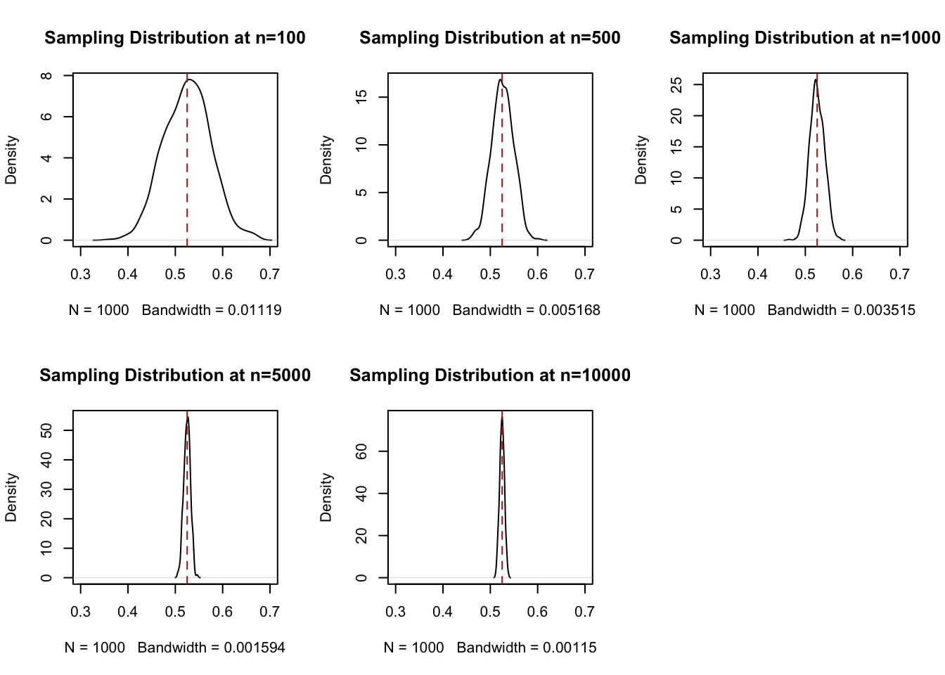
This is not necessarily crazy to you right now. But I want you to understand that this is wild. Each cross-section of this distribution is a normal (bell shaped) distribution that is centered on the expected value of the variable that we are sampling. The fact that these are normal distributions will become very important in a second, but what you need to know right now is that we (the computer) knows everything about a normal distribution: if you tell me what it’s mean and variance is, I can draw it exactly. And these are normal distributions!
We call each of these distributions a “sampling distribution”. This is one of the phrases you truly have to know and so really focus in at this moment. A sampling distribution is the distribution of all estimates (here, for a sample mean) for a given sample size. It is not a distribution of a particular sample, and it is not the distribution of the random variable we are sampling from. Rather, it is the theoretical distribution of all possible sample means, if we sampled and calculated those estimates a large number of times.
The sampling distributions above are descriptions of the simulation process we underwent: we made repeated samples of size 100, size 500 etc, and had the computer show us that the distribution of means look like at that \(n\).
The critical things is that these sampling distributions are also predictions of what will happen when we sample, say, 500 Pennsylvania voters on whether they will vote for Fetterman or Oz. The relative height of the sampling distribution tells us the probability of obtaining a sample mean (the proportion of people supporting Oz) at 30%, 40%, 63%, 74% etc.
Looking at the distribution for n=500, we are most likely to get a sample where the proportion supporting Fetterman is 52.5% (that’s true of any n, as we’ve seen!). It’s less likely that we get 55%. It’s almost impossible for us to get something above 60%.
Compare that to when n=10000, which is a sample of 10,000 voters. Again the most likely thing to happen is we have a sample mean of 52.5%. But this distribution is much tighter, and now anything above 55% is nearly impossible to get.
In other words, these sampling distributions are showing us that as the sample size increases, the relative size of the sampling error that we can have decreases.
We can describe the width of these sampling distributions via their variances:
var(binomial.sample[100,])
#> [1] 0.002448655
var(binomial.sample[500,])
#> [1] 0.0005225665
var(binomial.sample[1000,])
#> [1] 0.0002416901
var(binomial.sample[5000,])
#> [1] 4.973981e-05
var(binomial.sample[10000,])
#> [1] 2.587326e-05
But remember our original goal is to understand: If I am taking a sample of 100 people, how much would I expect to miss the true answer by, on average? I can’t sample 100 people 1000 times, so I need a way to estimate what these variances are before I take a sample. To get there we are going to need a bit of math.
5.3.3 A brief excursion into math
Yeah, yeah, yeah, this is a math-lite course, but it’s helpful at this point if we take a brief excursion into math to help us understand what is happening here in terms of sampling.
We have uncovered that, for any sample size, the sampling distribution of the sample mean is (1) normally distributed; (2) is centered on the true population mean; (3) Gets tighter as \(n\) increases.
What remains a mystery is this: can we know for a certain \(n\) what the sampling distribution of the sample mean will look like without simulation? In other words, can we be a little more specific about point (3) in a way that does not involve simulating data? If we can, we could recreate those cross-sections above for any random variable without all the R code.
We can in fact do that, and the way that we can is through understanding the expectation and variance operators.
The first thing to know is that the normal distribution is special because if we know the expected value and variance of a normal distribution we can draw it perfectly.
For example female height in the US is normally distributed with an expected value of 64 and a variance of 9. With that information alone I can get the computer to draw:
#(Note that the dnorm function wants sd, not var, so we do sqrt(9)=3 in that spot)
plot(seq(55,73,.01), dnorm(seq(55,73,.01), mean = 64, sd = 3), type="l",
     main="Female Height in the US", xlab="Height in Inches", ylab = "Probability of Occuring")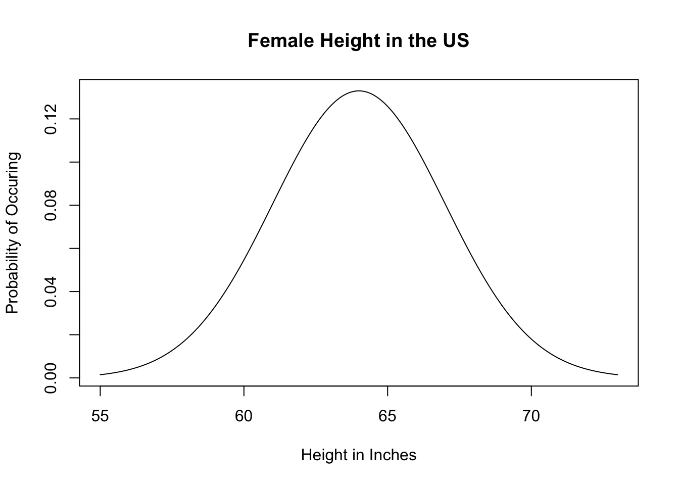
Because that’s the case, if we mathematically derive the expected value and variance of the sample mean we will be able to draw the (normally distributed) sampling distributions perfectly. So we want to know:
\[ E[\bar{X}] \]
and
\[ V[\bar{X}] \]
First we want to know:
\[ E[\bar{X}] = E[\frac{\sum_{i=1}^n X_i}{n} ] = ? \]
Before we start understanding how \(E[]\) as a mathematical operator works we can decompose what is inside the brackets. We can think about what is happening due to the summartion operator:
\[ =E[\frac{1}{n}*X_1 + X_2 + X_3 \dots X_n] \]
The expected value of a constant times a variable is the same as that constant times the expected value of the variable \(E[cX] = c*E[X]\).
Prove this to ourselves:
We treat \(n\) as a constant. That’s not to say we can’t have different N’s, but for a series of samples we hold constant the \(n\) we are drawing, which is what we care about here. To put it another way: if we are thinking about there being a random variable representing the sampling distribution, to generate a particular sampling distribution n must be fixed. So:
\[ \frac{1}{n}*E[X_1 + X_2 + X_3 \dots X_n] \]
The expected value operator is transitive, such that \(E[X+Z] = E[X] + E[Z]\). To prove this:
If that’s the case we can distribute the expectation operator:
\[ \frac{1}{n}*E[X_1] + E[X_2] + E[X_3] \dots E[X_n] \]
OK, what is the expected value of \(X_1\)? If I am sampling womens height (which is normally distributed with mean equal to 64), what would I guess the first height I will draw will be?. Don’t make this too hard. If the truth in the population is that the central tendency is 64, and I made you give me ONE number for a guess of what height the first woman would be, what would you say? 64! Our best guess for any observation is the expected value of the population. Therefore we can decompose this to
\[ \frac{1}{n}*E[X]+E[X]+E[X] +E[X] \dots E[X] \]
So now we are adding up \(n\) \(E[X]\) and dividing that by n. So that is just
\[ \frac{1}{n}*nE[X]\\ E[\bar{X}_n]=E[X] \] This tells us mathematically what we already knew, that the expected value of the sampling distribution of the sample mean is the expected value of the variable we are sampling from. Visually, this is the fact that each of the sampling distributions above are centered on the true population mean.
What is of more interest is:
\[ V[\bar{X}] = V[\frac{\sum_{i=1}^n X_i}{n} ] = ? \]
If we work this out, this will tell us what the expected width of a sampling distribution is for any given n.
We can do through a similar process, first decomposing what is inside the braces:
\[ V[\bar{X}_n]= V[\frac{1}{n}*(X_1 + X_2 + X_3 \dots +X_n)] \]
With the expectation operator we saw that \(E[cX_i]=c*E[X_i]\). This is not true for the variance operator. Instead: \(V[cX_i] = c^2V[X_i]\). Again we can prove this to ourselves
So to take out the constant \(n\):
\[ \frac{1}{n^2}*V[X_1 + X_2 + X_3 \dots X_n] \]
Similar to expectation: \(V[X+Z]=V[X]+V[Z]\) if X&Z are independent. Are \(X_1\) and \(X_2\) independent? Yes! That’s at the center of all of this, remember we assume our samples random, so one observation has nothing to do with the next.
So:
\[ \frac{1}{n^2}*V[X_1] + V[X_2] + V[X_3] \dots V[X_n] \]
Now this move is slightly weirder, but the variance of any given observation is also equal to the variance of the underlying random variable. This seems non-sensical. How can any individual observation have variance? The way to think about this is not “What is the variance of one individual estimate” it is: how much variation can we expect when we draw one sample from the random variable.
You can just believe me, but if we just take a sample of 1 from a random variable with a variannce of 1, 1000 times:
The variance is (approximately) 1. So with the knowledge that \(V[X_1]=V[X]\):
\[ \frac{1}{n^2}*V[X]+ V[X] + V[X] \dots V[X]] \]
That means we have:
\[ \frac{1}{n^2}*nV[X]\\ V[\bar{X}]= \frac{V[X]}{n} \]
The variance of our estimator is \(\frac{V[X]}{n}\): the variance of the random variable we are sampling from divided by the sample size.
This was a long way to go, so returning to our simulated samples:
par(mfrow=c(2,3))
plot(density(binomial.sample[100,]), main="Sampling Distribution at n=100", xlim=c(0.3,0.7))
abline(v=.525, col="firebrick", lty=2)
plot(density(binomial.sample[500,]), main="Sampling Distribution at n=500", xlim=c(0.3,0.7))
abline(v=.525, col="firebrick", lty=2)
plot(density(binomial.sample[1000,]), main="Sampling Distribution at n=1000", xlim=c(0.3,0.7))
abline(v=.525, col="firebrick", lty=2)
plot(density(binomial.sample[5000,]), main="Sampling Distribution at n=5000", xlim=c(0.3,0.7))
abline(v=.525, col="firebrick", lty=2)
plot(density(binomial.sample[10000,]), main="Sampling Distribution at n=10000", xlim=c(0.3,0.7))
abline(v=.525, col="firebrick", lty=2)
Mathematicaly we have shown the expected value of the sampling distribution is equal the the expected value of the thing we are sampling.
We have already seen that this is the case, but to confirm:
mean(binomial.sample[100,])
#> [1] 0.52544
mean(binomial.sample[500,])
#> [1] 0.52609
mean(binomial.sample[1000,])
#> [1] 0.524704
mean(binomial.sample[5000,])
#> [1] 0.5248978
mean(binomial.sample[10000,])
#> [1] 0.5246571
Approximately 52.5% at every level, as expected.
More interesting is the variance. These simulated sampling distributions have variances of:
var(binomial.sample[100,])
#> [1] 0.002448655
var(binomial.sample[500,])
#> [1] 0.0005225665
var(binomial.sample[1000,])
#> [1] 0.0002416901
var(binomial.sample[5000,])
#> [1] 4.973981e-05
var(binomial.sample[10000,])
#> [1] 2.587326e-05
The claim here is that we can derive these variances through the formula \(\frac{V[X]}{n}\).
\(V[X]\) is the variance of the thing we are sampling. The variance of a bernoulli random variable is the probability of success (\(\pi\)) multiplied by the probability of failure \((1-\pi)\).
So for a fair coin: \(V[X] = \pi*(1-\pi) = .5*.5 = .25\).
For our example here of the “Fetterman coin”: \(V[X] = .525 * .475 = .249\).
Which means that the variance of each sampling distribution should be \(\frac{.249}{n}\). Is that true?
#Calculated variances
.249/100
#> [1] 0.00249
.249/500
#> [1] 0.000498
.249/1000
#> [1] 0.000249
.249/5000
#> [1] 4.98e-05
.249/10000
#> [1] 2.49e-05
Yes! They are about the same.
Using some math, we have derived that the sampling distribution of the sample mean will be a normal distribution centered on the true population value and have a variance equal to the variance of the RV we are sampling from divided by the sample size.
Let’s plot those normal distributions against our empirical estimates to confirm that is true:
par(mfrow=c(2,3))
x <- seq(0,1,.0001)

plot(density(binomial.sample[100,]), main="Sampling Distribution at n=100", xlim=c(0.3,0.7))
points(x, dnorm(x, mean=.525, sd=.499/sqrt(100)), col="darkblue", type="l")
abline(v=.525, col="firebrick", lty=2)
plot(density(binomial.sample[500,]), main="Sampling Distribution at n=500", xlim=c(0.3,0.7))
points(x, dnorm(x, mean=.525, sd=.499/sqrt(500)), col="darkblue", type="l")
abline(v=.525, col="firebrick", lty=2)
plot(density(binomial.sample[1000,]), main="Sampling Distribution at n=1000", xlim=c(0.3,0.7))
points(x, dnorm(x, mean=.525, sd=.499/sqrt(1000)), col="darkblue", type="l")
abline(v=.525, col="firebrick", lty=2)
plot(density(binomial.sample[5000,]), main="Sampling Distribution at n=5000", xlim=c(0.3,0.7))
points(x, dnorm(x, mean=.525, sd=.499/sqrt(5000)), col="darkblue", type="l")
abline(v=.525, col="firebrick", lty=2)
plot(density(binomial.sample[10000,]), main="Sampling Distribution at n=10000", xlim=c(0.3,0.7))
points(x, dnorm(x, mean=.525, sd=.499/sqrt(10000)), col="darkblue", type="l")
abline(v=.525, col="firebrick", lty=2)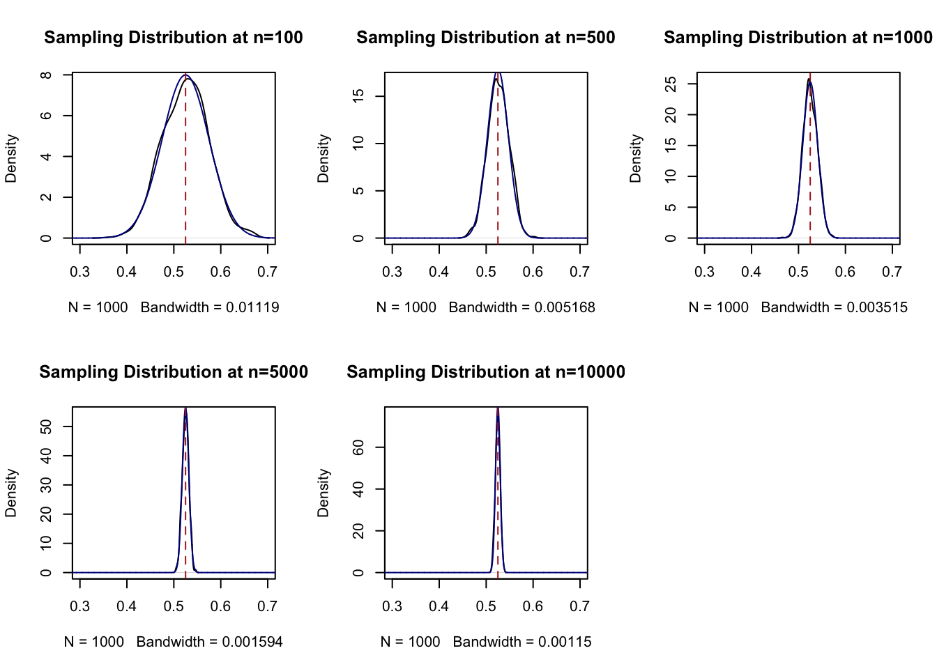
Fantastic! So before I take a sample and calculate a mean I can surmise that the distribution from which that mean is drawn from is normally distributed with mean equal to the expected value of the distribution I’m pulling from, and a variance that is equal to the variance of the distribution that I’m pulling from divided by the sample size.
The last part of this: that the sampling distribution is normally distributed with known parameters, is called the Central Limit Theorem.
In math:
\[ \bar{X_n} \leadsto N(\mu=E[X],\sigma^2 = V[X]/n) \]
The sampling distribution of the sample mean is normally distributed with \(\mu=E[X]\) and \(\sigma^2=\frac{v[x]}{n}\).
Together these things give us the third principle of sampling:
- The larger a sample the more likely our sample mean equals the expected value of the random variable we are sampling from (LLN).
- For any sample size, the expected value of the sample mean is the expected value of the random variable we are sampling from.
- The distribution of all possible estimates – the sampling distribution, – is normally distributed with it’s mean centered on the RV’s expected value, and variance determined by the variance of the RV and the sample size.
5.3.4 The Empirical Rule
So if I am going to sample 1000 Americans on whether they approve of Trump or not, and (for arguments sake) the true proportion who support Trump is 43%, then the sampling distribution of the sample mean will look like:
ev <- .43
var <- (.43*.57)/1000

plot(seq(.3,.56,.001), dnorm(seq(.3,.56,.001), mean = ev, sd = sqrt(var)), type="l",
     main="Sampling Distribution for Trump Approval",
     xlab="Proportion Approving Trump", ylab = "Probability of Getting a Sample with this Answer")
abline(v=.43, lty=2, col="firebrick")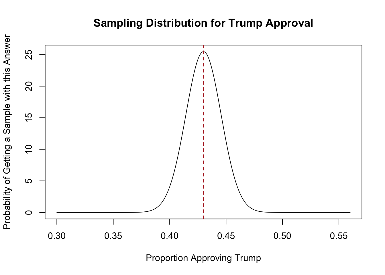
So before I go out and get a sample, I know that the most likely thing to happen is that I get a sample where the mean is 43%. It wouldn’t be crazy to get 45% or 41% approval. It is almost impossible that I would get 50% or 35% approval.
If instead I only sampled 500 people the sampling distribution would look different:
ev <- .43
var <- (.43*.57)/500

plot(seq(.3,.56,.001), dnorm(seq(.3,.56,.001), mean = ev, sd = sqrt(var)), type="l",
     main="Sampling Distribution for Trump Approval",
     xlab="Proportion Approving Trump", ylab = "Probability of Getting a Sample with this Answer")
abline(v=.43, lty=2, col="firebrick")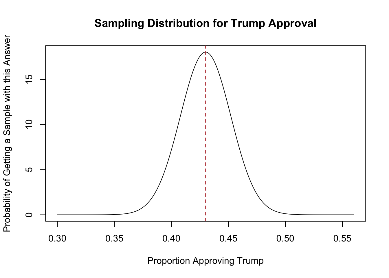
This sampling distribution is wider, telling me I’m more likely to get a trump approval of 40% or 47% etc.
The width of the sampling distribution is determined by the variance: \(\frac{V[X]}{n}\).
But to talk about the width of the sampling distribution we instead consider the square root of this variance (which is the standard deviation of the sampling distribution):
\[ \sqrt{V[\bar{X}]} = \sqrt{\frac{V[X]}{n}} = \frac{sd(X)}{\sqrt{n}} \]
We call this the standard error.
The standard deviation of the sampling distribution is the standard error. I have a tattoo of this on my arm it’s so important to remember.
Take a minute to think of how cool that equation is, by the way. What determines how wide of a sampling distribution we will have? The less variance in the random variable we are sampling, the smaller the sampling distribution. The larger the sample size, the smaller the sampling distribution (at a decreasing rate).
To get to a margin of error we have to do a bit more work.
In the above example where the Trump’s true population approval is 43% and we are taking a sample of 500 people, what are the two points that put 95% of the probability mass in the center of the distribution?
In other words, what are the two points that make this orange area equal 95%?
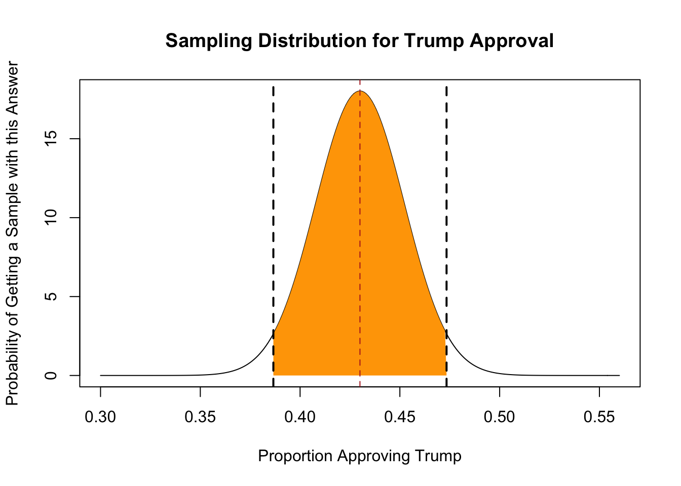
If you have done a little calculus you know that this is an integration problem. We are not goign to worry about the math here, because as discussed above the computer knows the shape of the normal distribution, and can do all the messy calculus for us. If there is 95% probability mass in the middle of the distribution, that means that there is 2.5% probability mass in both tails. Using R we get:
qnorm(.025, mean = ev, sd = sqrt(var))
#> [1] 0.3866055
qnorm(.025, mean = ev, sd = sqrt(var), lower.tail=F)
#> [1] 0.4733945
The two bounds are 38.6% and 47.3%. These are the two points that have in the middle of them 95% of the probability mass of the distribution.
I did not spend that much writing time on the previous explanation because I am now going to show you an incredible shortcut that means you don’t have to think about any of that.
What is the difference between the mean and the upper and lower bounds?
qnorm(.025, mean = ev, sd = sqrt(var)) - ev
#> [1] -0.04339451
qnorm(.025, mean = ev, sd = sqrt(var), lower.tail=F) - ev
#> [1] 0.04339451
They are 4.34% above and below the mean.
How many standard errors is 4.34. Remember, the standard error is the square root of the variance of the sampling distribution:
.0434/sqrt(var)
#> [1] 1.960212
Around 1.96 standard errors above and below the mean.
Here’s the helpful bit: for every normal distribution, plus or minus 1.96 standard errors around the mean contains 95% of the probability mass.
So if we instead had a sample size of 1000, the two points that contain 95% of the probability mass would be:
40% and 46%.
Just to confirm that:
So for any sampling distribution plus or minus 1.96 standard errors contains 95% of the probability mass. This is called the “Empirical Rule”.
5.3.5 Applying this to get the margin of error
In the above we started with the proposition that Trump’s approval rating is 43%, which allowed us to draw the sampling distribution for any sample size \(n\).
But that’s a bit stupid. If we know Trump’s approval rating going in we don’t need to do a survey at all.
So how do we apply this to get a margin of error for a poll.
Let’s say that we do a poll of 1000 people and we get a Trump approval rating of 45%. What we are going to do is to draw a sampling distribution around this number, pretending that it is the truth in the population.
To draw a sampling distribution we need the expected value, which we are saying is 45%, and the variance: \(\frac{V[X]}{n}\). We know \(n\), but to know \(V[X]\) we, again, need to know the truth in the population because the variance of a Bernoulli random variable is \(\pi*(1-\pi)\) where \(\pi\) is the probability of “success”, in this case approving of Donald Trump. And again, we don’t know that!
Here is where we get a move that is particular to survey research. Because we are often studying proportions, to calculate the standard error we just use a true probability of success of 50%, such that the standard error for a poll is always calculated as \(\sqrt{\frac{\pi*(1-\pi)}{n}}= \sqrt{\frac{.5*.5}{n}}\).
Why do we choose 50%? Because that is the largest the numerator of that equation can ever be. As with many other parts of science, we want to bias ourselves against over-confidence, so we start a standard error that is as big as possible for our given \(n\).
pi <- seq(0,1, .01)
one.minus.pi <- 1-pi
se <- sqrt((pi*one.minus.pi)/500)

plot(pi, se, type="l")
abline(v=.5, lty=2, col="firebrick")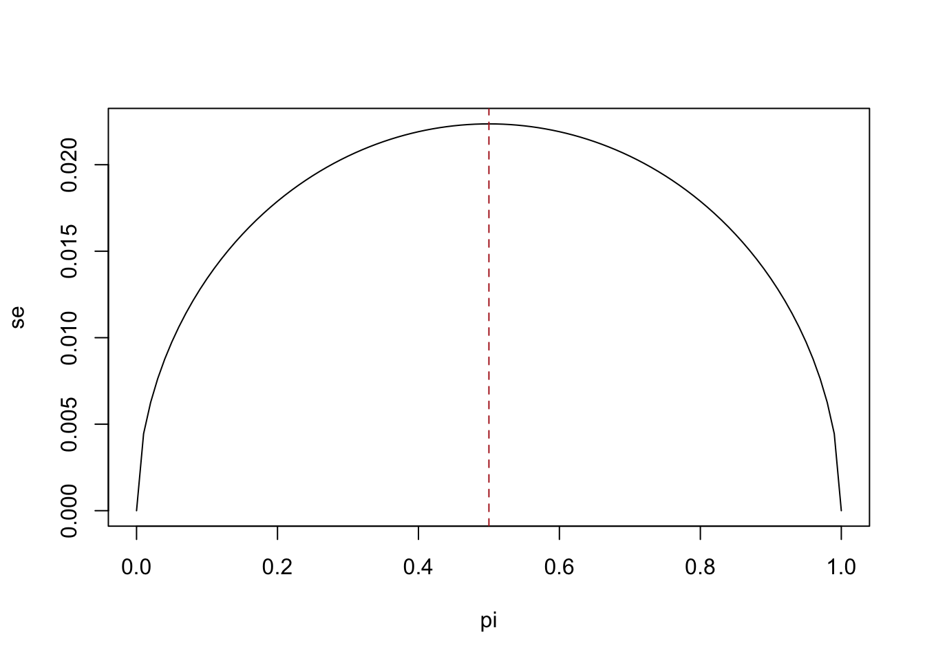
So we can draw a sampling distribution around our sample mean that looks like this:
ev <- .45
var <- (.5*.5)/1000

plot(seq(.3,.56,.001), dnorm(seq(.3,.56,.001), mean = ev, sd = sqrt(var)), type="l",
     main="Sampling Distribution for Trump Approval",
     xlab="Proportion Approving Trump", ylab = "Probability of Getting a Sample with this Answer")
abline(v=.45, lty=2, col="firebrick")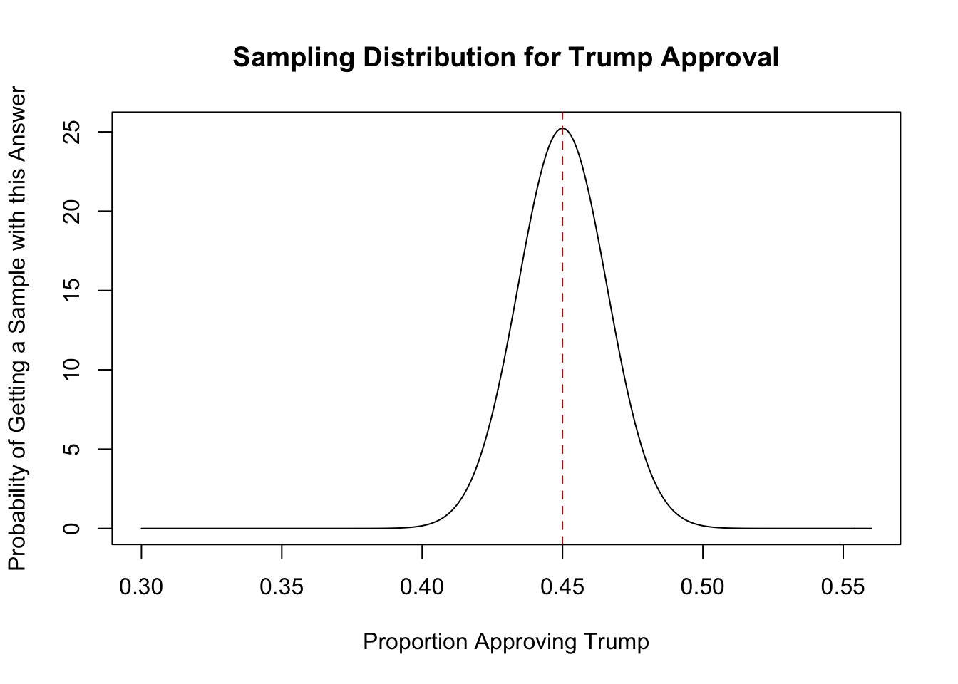
From there, we can put the same 95% interval around this percentage:
1.96*sqrt(var)
#> [1] 0.03099032
Our 95% interval is plus or minus 3.1 percentage points around our sample proportion.
This is a bit odd, where now we are putting this confidence interval around our sample mean. How does this help us understand what is likely or plausible for the truth about Trump’s approval rating?
When we construct a confidence interval in this way – put the appropriately sized sampling distribution around our sample proportion and calculate the area where 95% of estimates would lie – 95% of the time the confidence interval will include the true population proportion:
moe <- sqrt((.5*.5)/1000)

result <- NA

for(i in 1:10000){
sample <- rbinom(1000, 1, .43)
prop <- mean(sample)
low <- prop - 1.96*moe
high <- prop + 1.96*moe

#Test to see whether truth is in interval
result[i] <- low<=.43 & high>=.43
}

mean(result)
#> [1] 0.9513
So for a 95% confidence interval the technically correct thing to say is: 95% of similarly constructed confidence intervals contain the true population parameter.
This is a persnickety stats thing to say, and it’s easier to say “There is a 95% chance this confidence interval contains the truth”. They think about things this way because we think that the truth (here Trump’s approval rating) is a real, fixed thing. The two bounds to our confidence interval are also two, real, fixed things. So – again, technically – the truth is either in the confidence interval or not in the confidence interval. There is no probability to it at all.
However, given that we aren’t sure if our confidence interval contains the true population parameter or not, and 95% of confidence intervals contain the true population parameter, I am fine with the estimation that “there is a 95% chance that this confidence interval contains the truth.”
So the margin of error is the 95% confidence interval derived from a sampling distribution with standard error \(\sqrt{\frac{.25}{n}}\). This leads back to the original equation for a margin of error, which you should now fully understand:
\[ MOE = 1.96 * \sqrt{\frac{.5*.5}{n}} \]
We could technically apply a more accurate margin of error to each proportion in our sample by subbing out the \(.5*.5\) for the particular proportion we are calculating the confidence interval for. This would have a non-significant effect on proportions very close to 0 or 1 because those have smaller variances: \(.99*.01 = .0099\), for example. But because we only report one margin of error for the whole poll, we go for the number that is as large as possible, which is for a proportion of 50%.
5.4 What is it good for?
Remember that this margin of error only represents the error in our poll that is due to random sampling, it does not take into account measurement error, non-coverage error, processing error etc.
Still, this provides a reasonable baseline of what we can expect the error to be for a poll of the size that we are doing.
It’s also important to remember that this is the margin of error around each proportion in the survey. If we are comparing two proportions each of those has a margin of error.
If a poll has a margin of error of plus or minus 3, and the two candidates have proportions of 52 and 48, should we be confident that the real difference is not 0? No! We should not be confident at all about that, because candidate 1 has a confidence interval of 49-55 and candidate two has a confidence interval of 45-51. Standard practice is to say “the confidence interval should be doubled when looking at the difference between two proportions, like the difference between candidates”. That’s a fine rule of thumb though it is not 100% statistically true.
5.5 Questions
If I am doing an RBS survey of registered voters, what are the elements and what is the sampling frame? What are some possible sources of coverage error?
Some people may be listed twice in the voter file if they move states. Why is this a possible source of coverage error?
I am doing a survey where 5% of people are uncovered. Those people have an opinion that is 10 percentage points different than those who are covered. What is the coverage error of this survey?
What is the margin of error of a poll of 500 people?
Describe the relationship between a sampling distribution and the margin of error.
How would you explain to a person who has never taken a statistics class what a “standard error” is, and why it’s important to survey research?
Is the following statement true? “There is a 95% chance the margin of error contains the true value in the population”.