6 Sampling II
6.1 Finite Population Corrections
One of the hallmarks of the central limit theorem is that it operates well regardless of the size of the population from which you are sampling from.
For example, the standard error for a poll of 1000 people from a population of 1 million people should have a standard error of \(\sqrt{\frac{.25}{1000}} = 0.016\):
pop <- rbinom(1E6, 1, .5)
means <- NA

for(i in 1:10000){
  means[i] <- mean(sample(pop, 1000))
}
sd(means)
#> [1] 0.01572775
And the same is true for a poll of 1000 people from a population of 100 million people:
pop <- rbinom(1E8, 1, .5)
means <- NA

for(i in 1:10000){
  means[i] <- mean(sample(pop, 1000))
}
sd(means)
#> [1] 0.01598734
This is why we can use the same sized sample to study Canada, the US, and China.
But surely this logic breaks down eventually. If we have a population of 1001 people and do a survey of 1000 people our standard error is not going to be .016:
pop <- rbinom(1001, 1, .5)
means <- NA

for(i in 1:10000){
  means[i] <- mean(sample(pop, 1000))
}
sd(means)
#> [1] 0.0005000082
Way smaller!
We can mathematically determine this using a finite population correction. To get the correct margin of error we can calculate the standard error with a correction factor:
\[ \sqrt{\frac{N-n}{N-1}} *\sqrt{\frac{.25}{n}} \]
Where \(N\) is the size of the population and \(n\) is the sample size.
So for the above case where we had a population of 1001 and a sample size of 1000:
\[ SE_{f} = \sqrt{\frac{1001-1000}{1001-1}} *\sqrt{\frac{.25}{1000}}\\ SE_{f} = \sqrt{\frac{1}{1000}} *0.016\\ SE_{f} = .0005 \]
Which is just about what we got.
Whenever our sample size starts to approach the population size we should apply this correction to get a more accurate standard error.
However, looking at the correction it should be clear that for a constant sample size \(n\), as \(N\) gets bigger the correction rapidly converges on 1.
Here is what the correction looks like for a sample size of 1000 at different population levels. (Note the non-linear x-axis)
pop <- 10^seq(3,7,0.1)

correction <- sqrt((pop-1000)/(pop-1))

plot(log10(pop), correction, axes=F, pch=16,
     xlab="Population Size",
     ylab="Finite Population Correction")
axis(side=1, at = 3:7, labels = 10^(3:7), )
axis(side=2, las=2)
abline(h=1, lty=2, col="firebrick")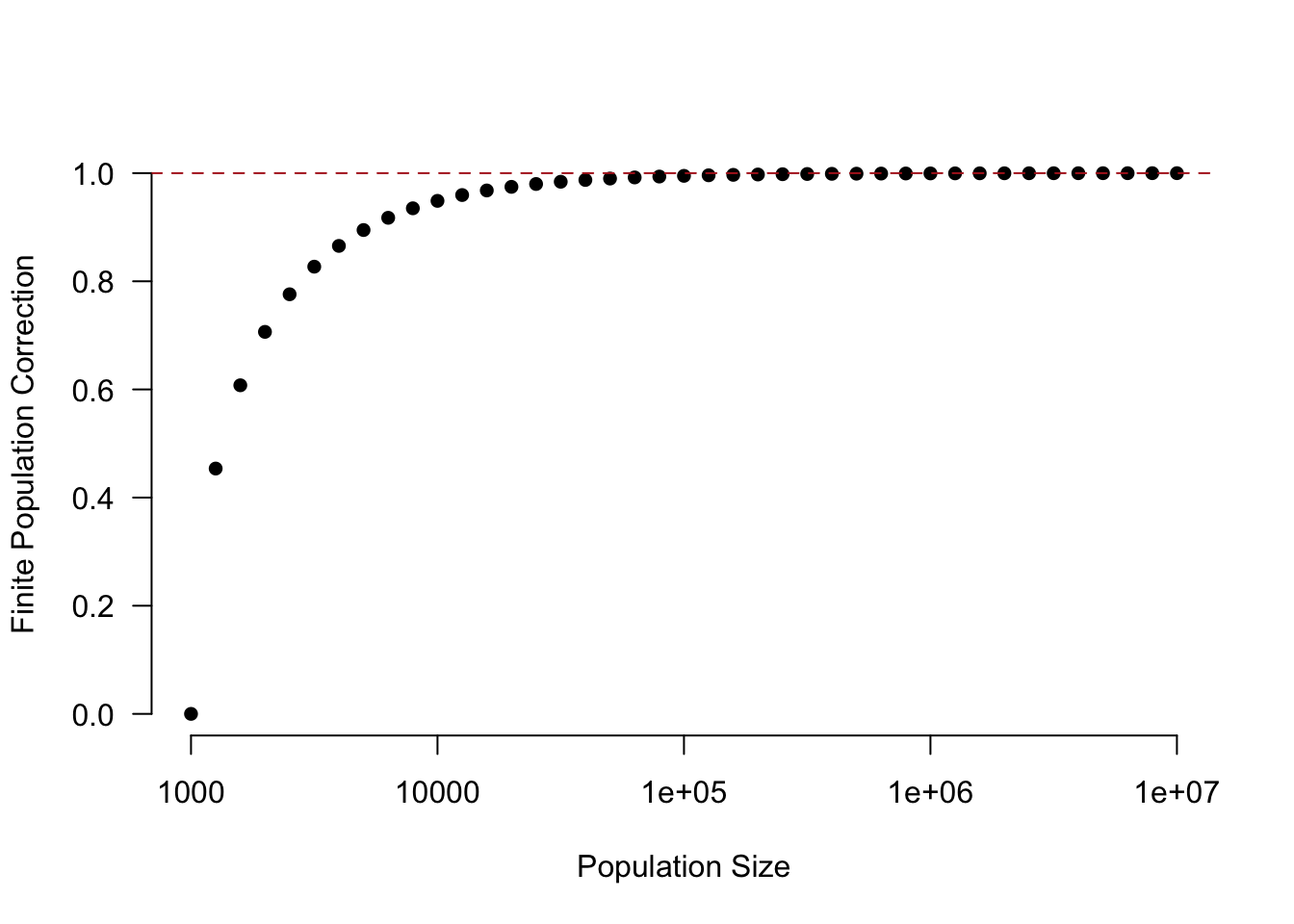
For a sample size of 1000 once our population gets to around 100,000 the finite population correction is effectively 1. In other words, once we are at this level then there is no point in worrying about it anymore. That’s why when we think about doing a survey of 1000 people in Canada (approx 30 million people), the US (approx 330 million people), and China (approx 1.5 billion people) there is no need to apply the finite population correction, because it would be approximately 1 in all of these cases.
6.2 Cluster Sampling
This topic will not be on the midterm.
Simple random sampling is the gold standard because of the statistical properties uncovered in the frist part of this chapter, but the big downside is the cost. This is particularly (or primarily) true when considering face-to-face surveys.
Let’s say we want to do a study on a population of school children where there are 1000 students in 40 classrooms, with each classroom having 25 students. We want a sample of 100 students.
This is code to set up this data. Don’t worry too much about it:
set.seed(2105)
#Cluster sampling simulation
library(tidyverse)
#> Warning: package 'ggplot2' was built under R version 4.4.3
#> ── Attaching core tidyverse packages ──── tidyverse 2.0.0 ──
#> ✔ dplyr     1.1.4     ✔ readr     2.1.5
#> ✔ forcats   1.0.0     ✔ stringr   1.6.0
#> ✔ ggplot2   4.0.1     ✔ tibble    3.3.0
#> ✔ lubridate 1.9.4     ✔ tidyr     1.3.1
#> ✔ purrr     1.2.0
#> ── Conflicts ────────────────────── tidyverse_conflicts() ──
#> ✖ dplyr::filter() masks stats::filter()
#> ✖ dplyr::lag()    masks stats::lag()
#> ℹ Use the conflicted package (<http://conflicted.r-lib.org/>) to force all conflicts to become errors
# 40 classrooms of 25 people

classroom <- sort(rep(1:40,25))
student <- rep(1:25,40)

population <- cbind.data.frame(classroom, student)

#Randomly assign a latent level to each classroom
classroom <- 1:40
latent.level <- runif(40,-3.4,3.4)
latent <- cbind.data.frame(classroom, latent.level)

population |>  left_join(latent) -> population
#> Joining with `by = join_by(classroom)`

#Generate student outcomes - Case 1, outcomes closely linked to latent levels
population$individual.prob <- population$latent.level + rnorm(nrow(population), mean=0, sd=2)
population$outcome <- if_else(pnorm(population$individual.prob)>.5,T,F)
population |>
  group_by(classroom) |>
  summarize(mean(outcome))
#> # A tibble: 40 × 2
#>    classroom `mean(outcome)`
#>        <int>           <dbl>
#>  1         1            0.12
#>  2         2            0.48
#>  3         3            0.88
#>  4         4            0.96
#>  5         5            0.12
#>  6         6            0.4
#>  7         7            0.92
#>  8         8            0.04
#>  9         9            0.92
#> 10        10            0.44
#> # ℹ 30 more rows
If we randomly selected 100 students to interview we will have to visit a lot of school for face-to-face interviews.
For example here is one random sample:
random.sample <- population[sample(1:nrow(population), 100),]
sort(unique(random.sample$classroom))
#>  [1]  2  3  4  5  6  7  8  9 10 12 13 15 16 18 19 20 21 22
#> [19] 23 24 25 26 27 28 29 30 31 32 33 34 35 36 37 38 39 40
We would have to visit all of those classrooms! That’s a lot of expense.
But if we do that the sampling principles will apply from above. The sample mean will be unbiased, and the standard error will be \(\sqrt{\frac{.25}{100}}\).
mean(random.sample$outcome)
#> [1] 0.47

#Calculate standard error
sqrt(.25/100)
#> [1] 0.05

#Estimate standard error through sampling:

sample.mean <- NA

for(i in 1:1000){
  sample.mean[i] <- mean(sample(population$outcome, 100))
}
#Unbiased
mean(population$outcome)
#> [1] 0.491
mean(sample.mean)
#> [1] 0.49074
#Standard Error (Approximately correct)
sd(sample.mean)
#> [1] 0.04659424
So that works great, but if we want to save money we can alternatively get our sample of 100 people by visiting 4 schools and interviewing all 25 students in the classroom. This is way cheaper to do.
Critically, the means of the different classrooms are all quite different. This is not surprising, some schools are better than others and we expect outcomes to be correlated within classrooms. If this measure is passing a test, for example, we expect all students to do well in some classrooms, and all students to do poorly in others.
Here are the various classroom means:
population |>
  group_by(classroom) |>
  summarize(mean(outcome))
#> # A tibble: 40 × 2
#>    classroom `mean(outcome)`
#>        <int>           <dbl>
#>  1         1            0.12
#>  2         2            0.48
#>  3         3            0.88
#>  4         4            0.96
#>  5         5            0.12
#>  6         6            0.4
#>  7         7            0.92
#>  8         8            0.04
#>  9         9            0.92
#> 10        10            0.44
#> # ℹ 30 more rows
Let’s simulate what that would look like to sample 4 classrooms and interview all the students in that classroom
#Do it once first:

sample <- population[population$classroom %in% sample(1:40, 4),]
table(sample$classroom)
#>
#>  3 17 24 32
#> 25 25 25 25
mean(sample$outcome)
#> [1] 0.53

#Now simulate doing this many times:

sample.means <- NA
for(i in 1:1000){
  sample <- population[population$classroom %in% sample(1:40, 4),]
  sample.means[i] <- mean(sample$outcome)
}


sd(sample.means)
#> [1] 0.1473865

plot(density(sample.means), main="Cluster Sampling Distribution")
abline(v=mean(sample.means), lty=2, col="darkblue", lwd=3)
abline(v=.49, lty=2, col="firebrick")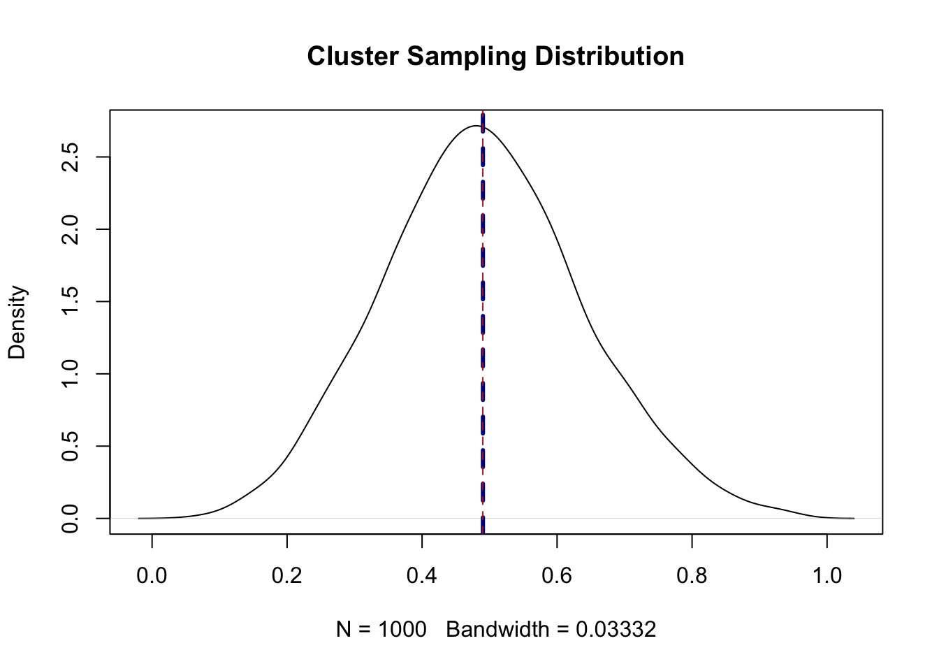
Note that the sample mean here is just the simple mean of the 100 people. This is because each classroom has the same number of people in it. If this was not the case we would have to calculate a weighted mean.
What can we see in this sampling distribution? First of all, the mean of the 1000 sample means we calculated using this method is right on top of the true population mean. So this is an unbiased method of estimating the sample mean. That’s good!
But what about the standard error. As a reminder, the standard error for a simple random sample of 100 people is \(\sqrt{\frac{.25}{100}} = .05\).
Here the standard error is:
sd(sample.means)
#> [1] 0.1473865
15 percentage points! Nearly three times larger.
Look what the simple random sample sampling distribution looks like laid on top of this sampling distribution:
plot(density(sample.means), main="Cluster Sampling Distribution")
abline(v=mean(sample.means), lty=2, col="darkblue", lwd=3)
abline(v=.49, lty=2, col="firebrick")
points(seq(0,1,.001), dnorm(seq(0,1,.001), mean=.49, sd=.05), col="orange", type="l")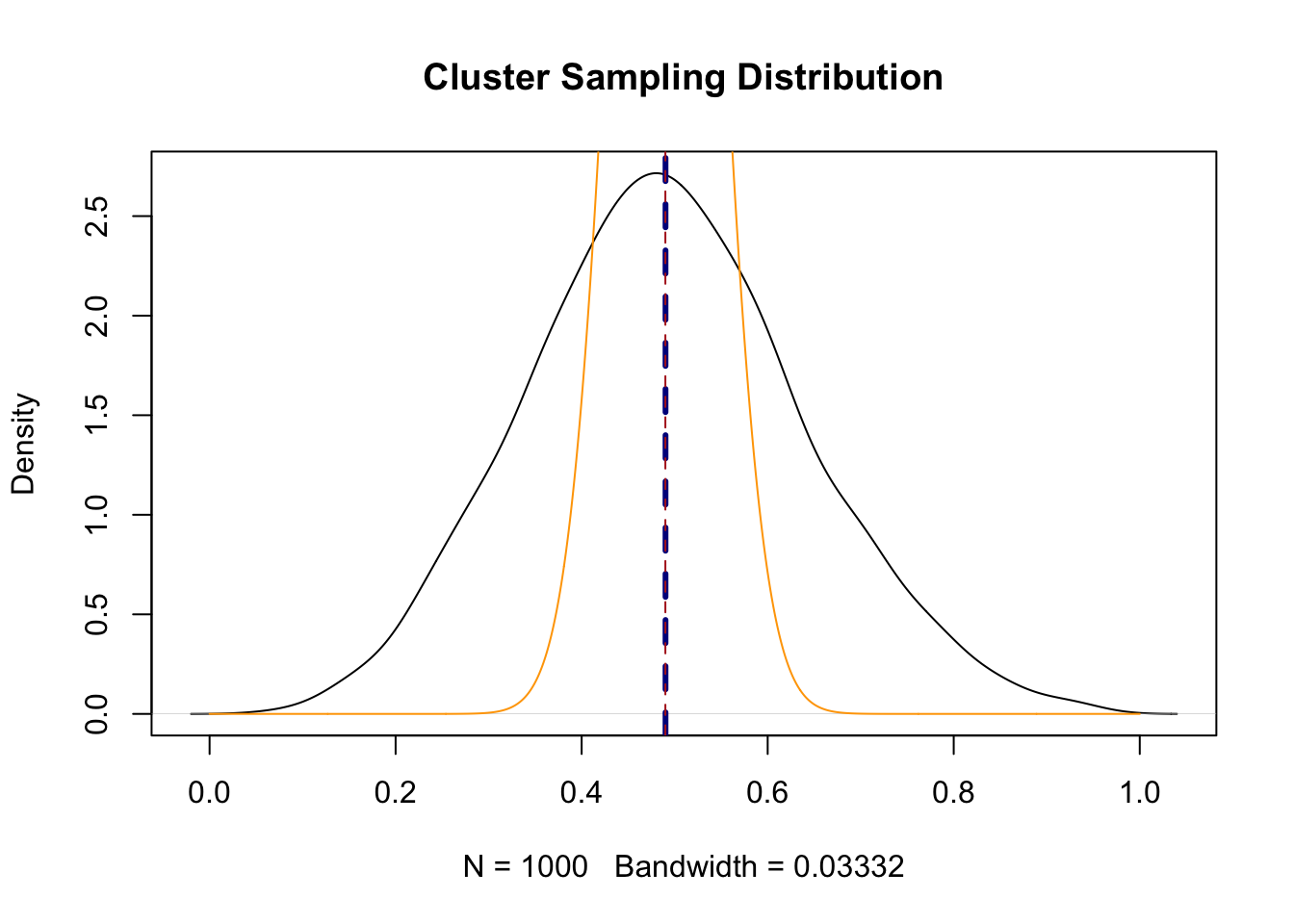
Ridiculously skinnier.
So what is happening here?
Nothing is free! While cluster sampling is much more cost effective, it comes at the expense of a much higher standard error. What is the intuition behind this? Because outcomes are correlated within classrooms, when we sample all the students from one classroom we get relatively similar answers. Sometimes in our random sample of 4 classrooms we are going to to get all rich classroooms, sometimes we are going to get poor classrooms. In expectation we get the right balance and that’s why the sampling distribution is centered on the right spot. But we also expect a lot of variance from sample to sample.
Can we calculate this expected variance before we set out to sample? Yes, by calculating:
\[ se_c(\bar{y}) = \sqrt{\frac{s_a^2}{a}} \]
Where \(a\) denotes classrooms. In other words, this is the between classroom variance divided by the number of classrooms we are sampling.
So in this case the between classroom variance in the population is:
population |>
  group_by(classroom) |>
  summarise(classroom.means = mean(outcome)) |>
  summarise(var(classroom.means))
#> # A tibble: 1 × 1
#>   `var(classroom.means)`
#>                    <dbl>
#> 1                  0.100
Around .1. So we expect the standard error to be:
sqrt(.1/4)
#> [1] 0.1581139
.15, which is exactly what we got through simulation.
Can this variance be made smaller? Sort of! Looking at the equation, what can be done to make cluster sampling more efficient?
First of all, if the between classroom variance is smaller, then the standard error will be smaller. In other words, the more similar clusters are to one another, the better cluster sampling does in approximating simple random sampling.
The between classroom variance in the initial example was .1, or 10 percentage points.
I can re-generate the data with a smaller between classroom variance:
set.seed(2105)
#Cluster sampling simulation
library(tidyverse)
# 40 classrooms of 25 people

classroom <- sort(rep(1:40,25))
student <- rep(1:25,40)

population2 <- cbind.data.frame(classroom, student)

#Randomly assign a latent level to each classroom
classroom <- 1:40
latent.level <- runif(40,-3.4,3.4)
latent <- cbind.data.frame(classroom, latent.level)

population2 |>  left_join(latent) -> population2
#> Joining with `by = join_by(classroom)`

#Generate student outcomes - Case 1, outcomes closely linked to latent levels
population2$individual.prob <- population2$latent.level + rnorm(nrow(population2), mean=0, sd=10)
population2$outcome <- if_else(pnorm(population2$individual.prob)>.5,T,F)
population2 |>
  group_by(classroom) |>
  summarize(classroom.means = mean(outcome)) |>
  summarize(var(classroom.means))
#> # A tibble: 1 × 1
#>   `var(classroom.means)`
#>                    <dbl>
#> 1                 0.0185
Now the between classroom variance is just under 2 percantage points. That means we expect the standard error of the cluster estimator to be:
sqrt(.018/4)
#> [1] 0.06708204
And if we simulate:
sample.means <- NA
for(i in 1:1000){
  sample <- population2[population2$classroom %in% sample(1:40, 4),]
  sample.means[i] <- mean(sample$outcome)
}
sd(sample.means)
#> [1] 0.06478761
We get approximately the same answer.
That’s a bit stupid, because we don’t control the between classroom variance we can’t really put that as part of a “plan” for lowering the standard error.
What we can do is to sample more classrooms. All the equation for the standard error for the cluster sample cares about is the number of clusteres sampled. So instead of 4 classrooms where we interview all 25 people, let’s do 10 classrooms where we interview 10 people each. This should make the standard error:
sqrt(.1/10)
#> [1] 0.1
To simulate (we are back to the original population):
sample.means <- NA
for(i in 1:1000){
sample <- population[population$classroom %in% sample(1:40, 10) &
                        population$student %in% sample(1:25,10),]
  sample.means[i] <- mean(sample$outcome)
}
sd(sample.means)
#> [1] 0.09173339
About the same! Obviously this would be more expensive then visiting 4 classrooms and interviewing all 25 students in those classrooms, but still less expensive then doing a simple random sample.
6.3 Stratified Sampling
This topic will not be on the midterm.
Another, similar variation on sampling is stratified sampling. This can seem similar to cluster sampling because we are explicitly splitting the population into groups and then sampling them, but in contrast, stratified random sampling actually improves the efficiency of our design (i.e. leads to lower standard error and margins of error).
Consider the following population we might want to study. There are 100,000 people in this population and for each they have a value for whether they would vote for a Republican candidate (T) or not (F). Additionally, we know for each of these people’s race and education level, such that we can split the population into 4 groups based on whether they are white, or not; and whether they have a college education, or not.
head(pop)
#>   vote.republican        race.education
#> 1            TRUE     White non-college
#> 2            TRUE     White non-college
#> 3           FALSE Non-white non-college
#> 4            TRUE         White college
#> 5           FALSE     White non-college
#> 6           FALSE Non-white non-college
mean(pop$vote.republican)
#> [1] 0.50135

pop |>
  group_by(race.education) |>
  summarise(size = (n()/100000)*100,
            rep.percent = mean(vote.republican)*100)
#> # A tibble: 4 × 3
#>   race.education         size rep.percent
#>   <fct>                 <dbl>       <dbl>
#> 1 Non-white non-college  21.8        41.4
#> 2 Non-white college      18.4        16.8
#> 3 White non-college      23.1        79.1
#> 4 White college          36.7        53.8
Critically: the 4 groups created by the crossover of race and education are of different sizes, and the people within those groups have different vote choices.
Let’s say we take a simple random sample of 400 people from this population. Our expectation is that the standard error for this group will be \(\sqrt{\frac{.25}{400}}= 0.025\) or 2.5%.
sample.means.srs <- NA

for(i in 1:1000){
  sample.means.srs[i] <- mean(pop$vote.republican[sample(1:nrow(pop), 400)])
}

sd(sample.means.srs)
#> [1] 0.02468473

plot(density(sample.means.srs), main="Sampling Distribution")
abline(v=.501, lty=2, col="firebrick", lwd=2)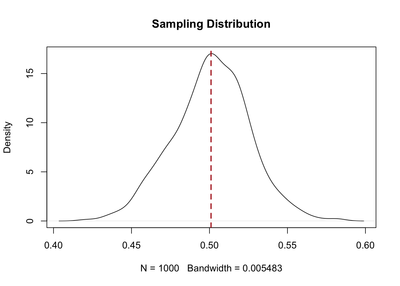
In line with what we know about simple random sampling, the sampling distribution for a simple random sample is normally distributed, with the standard error determined by the sample size, and centered on the true population proportion (50.1%).
But in this case we also have these very informative groups that we know have very different vote choices.
Let’s try a different sampling method. Instead of taking a simple random sample, I am going to take a sample of 100 from each of the 4 “stratum”, in this case the 4 unique combinations of race and education we have listed.
sample.means.strat1 <- NA

for(i in 1:1000){
  sample<- bind_rows(pop |> filter(race.education=="Non-white non-college") |>  slice_sample(n=100),
                                          pop |> filter(race.education=="Non-white college") |>  slice_sample(n=100),
                                          pop |> filter(race.education=="White non-college") |>  slice_sample(n=100),
                                          pop |> filter(race.education=="White college") |>  slice_sample(n=100))
  sample.means.strat1[i] <- mean(sample$vote.republican)
}
plot(density(sample.means.srs), main="Sampling Distribution")
points(density(sample.means.strat1), type="l", col="blue")
abline(v=.501, lty=2, col="firebrick", lwd=2)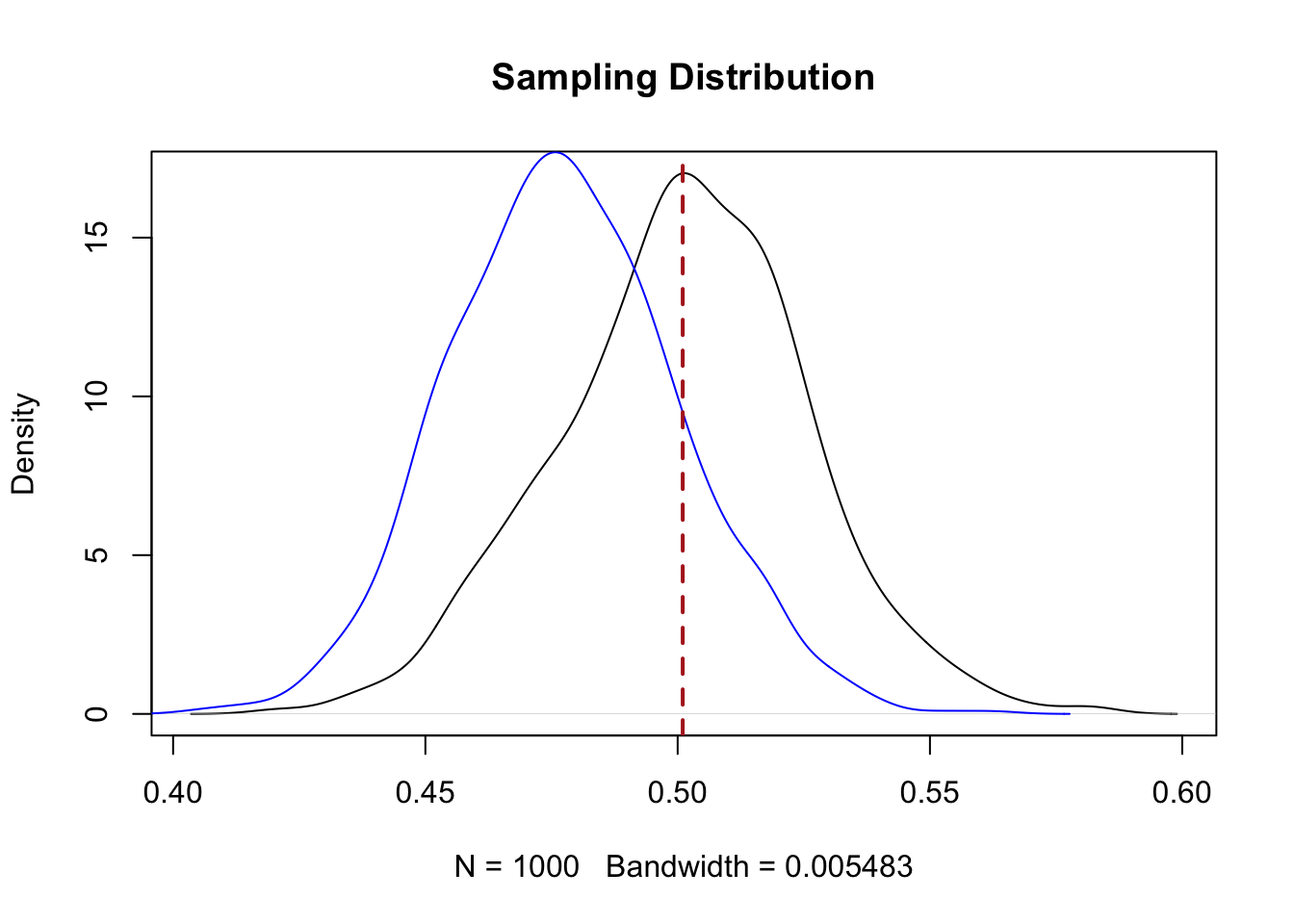
sd(sample.means.strat1)
#> [1] 0.02251625
What do we see here? First, the standard error on this sampling distribution is lower. Visually, we see that the sampling distribution is wider and taller than the simple random sample sampling distribution.
But that’s not our main concern here: the sampling distribution is in the wrong place!
We know that the population mean is 50.1% voting Republican, but here our sampling distribution is centered on:
mean(sample.means.strat1)
#> [1] 0.47752
47.8%.
Why is this happening?
Remember, these 4 strata are not equally sized in the population. When we did our sampling we had 100 people from each group. So when we calculated the mean we were assuming each of these groups were exactly a quarter of the population, which they are not!
How can we address this?
Let’s consider the strata: “non-white college”. The true number of these people in our population is:
18,392 people out of 100,000 population, or 18.3%.
If we think about the probability of each of those people being selected into our sample of 100, it is \(p_s = \frac{100}{18392}\).
If we consider the white-college strata:
There the probability of selection is \(p_s = \frac{100}{36725}\).
Individuals from larger strata have a lower probability of selection, while individuals from smaller strata have a higher probability of selection. This throws off the mean that we calculate, giving unproportionate weight to those individuals who are in smaller strata.
How do we fix this? We can do so by weighting each strata by the inverse of the selection probability.
So for one sample:
  sample<- bind_rows(pop |> filter(race.education=="Non-white non-college") |>  slice_sample(n=100),
                                          pop |> filter(race.education=="Non-white college") |>  slice_sample(n=100),
                                          pop |> filter(race.education=="White non-college") |>  slice_sample(n=100),
                                          pop |> filter(race.education=="White college") |>  slice_sample(n=100))

  #Assign weights
  sample |>
    mutate(weight = case_when(race.education=="Non-white non-college" ~ 1/(100/21750),
                              race.education=="Non-white college" ~ 1/(100/18392),
                              race.education=="White non-college" ~1/(100/23133),
                              race.education=="White college" ~ 1/(100/36725))) -> sample

weighted.mean(sample$vote.republican, w=sample$weight)
#> [1] 0.5150988
And now simulating that a large number of times:
sample.means.strat2 <- NA

for(i in 1:1000){
    sample<- bind_rows(pop |> filter(race.education=="Non-white non-college") |>  slice_sample(n=100),
                                          pop |> filter(race.education=="Non-white college") |>  slice_sample(n=100),
                                          pop |> filter(race.education=="White non-college") |>  slice_sample(n=100),
                                          pop |> filter(race.education=="White college") |>  slice_sample(n=100))

  #Assign weights
  sample |>
    mutate(weight = case_when(race.education=="Non-white non-college" ~ 1/(100/21750),
                              race.education=="Non-white college" ~ 1/(100/18392),
                              race.education=="White non-college" ~1/(100/23133),
                              race.education=="White college" ~ 1/(100/36725))) -> sample

sample.means.strat2[i] <- weighted.mean(sample$vote.republican, w=sample$weight)
}

plot(density(sample.means.srs), main="Sampling Distribution")
points(density(sample.means.strat1), type="l", col="blue")
points(density(sample.means.strat2), type="l", col="orange")
abline(v=.501, lty=2, col="firebrick", lwd=2)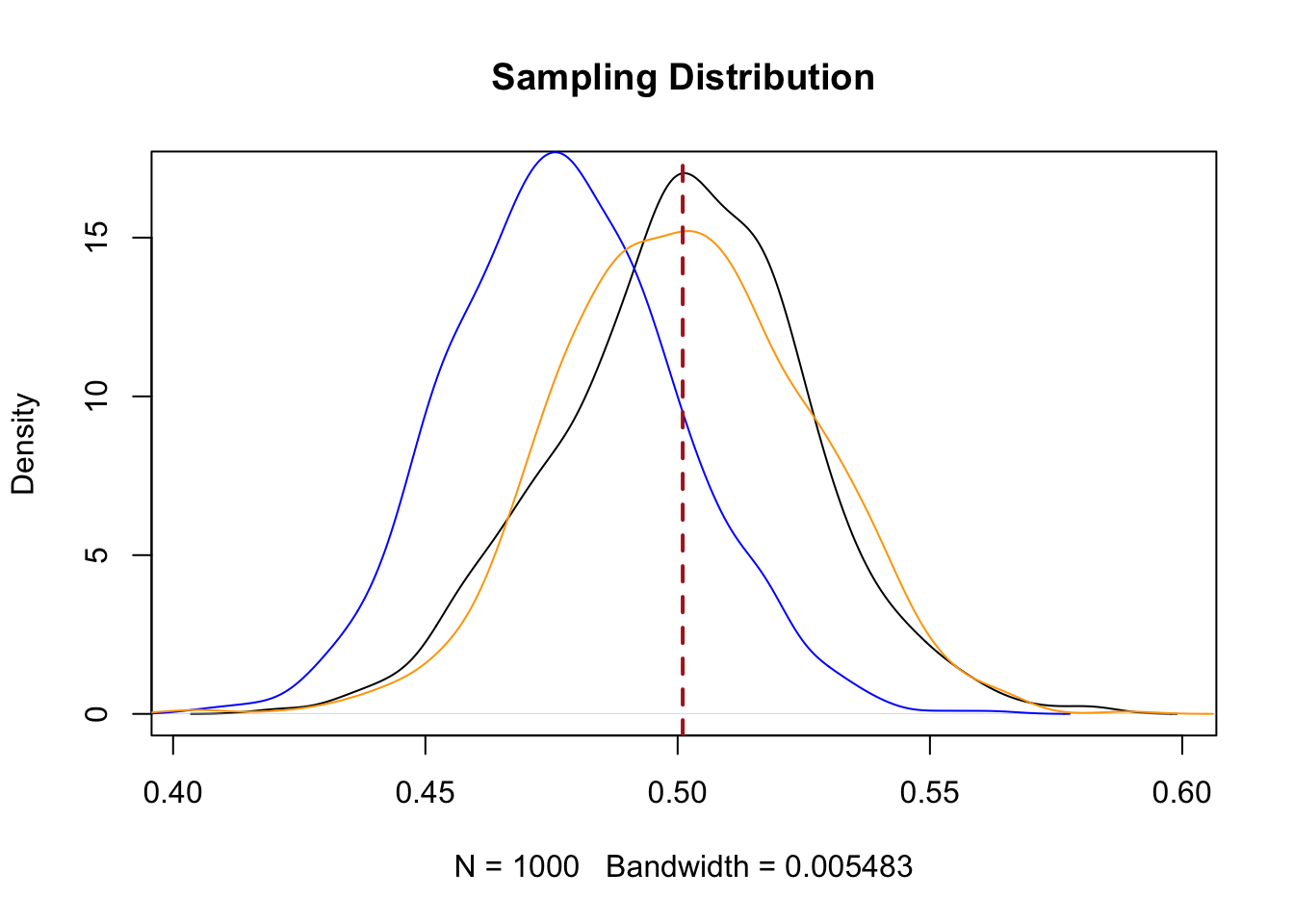
sd(sample.means.strat2)
#> [1] 0.02480766
Screaming, crying, throwing-up. Ok, so, weighting the strata so that they are properly sized when taking the mean has centered our sampling distribution on the correct place, but at the expense of the gains in efficiency we initially achieved. Now our sampling distribution looks just like the one we got through random sampling.
So that’s not worth doing.
What is worth doing is thinking about the unequal group size on the front end of sampling. Instead of sampling 100 people from each group, instead what we want to do is to sample in proportion to the size of the group in the population. So using the actual proportions in the population, we can determine the proportion of the 400 person sample that needs to come from that group. With strict proportional sampling (i.e. we nail it and have every group perfectly sized) there is also no need to estimate a weighted mean, because the groups are already in their correct proportions!
#Sample sizes:
round(400*.21750)
#> [1] 87
round(400*.18392)
#> [1] 74
round(400*.23133)
#> [1] 93
round(400*.36725)
#> [1] 147

sample.means.strat3 <- NA

for(i in 1:1000){
  sample<- bind_rows(pop |> filter(race.education=="Non-white non-college") |>  slice_sample(n=87),
                                          pop |> filter(race.education=="Non-white college") |>  slice_sample(n=74),
                                          pop |> filter(race.education=="White non-college") |>  slice_sample(n=93),
                                          pop |> filter(race.education=="White college") |>  slice_sample(n=147))
  sample.means.strat3[i] <- mean(sample$vote.republican)
}
plot(density(sample.means.srs), main="Sampling Distribution")
points(density(sample.means.strat1), type="l", col="blue")
points(density(sample.means.strat2), type="l", col="orange")
points(density(sample.means.strat3), type="l", col="magenta")

abline(v=.501, lty=2, col="firebrick", lwd=2)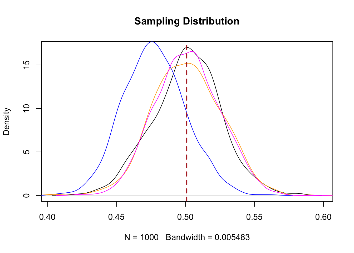
sd(sample.means.strat3)
#> [1] 0.02341987
Here we have an unbiased estimate of the population mean and a standard error that is smaller than what we get from simple random sampling.
Why is it smaller. Unlike cluster sampling we are sampling from the whole population here, just split into informative chunks. We aren’t going to miss any segments of the population. Because the people within those chunks are similar to one another, sampling from within them produces lower variance then if we have a simple random sample.
Can we estimate this standard error without simulation? Yes, we can, though I don’t really want to go all the way through calculating it.
We get this standard error by calculating:
\[ se_{strat} = \sum_s W_S^2*\frac{\sigma^2_s}{n_s} \]
Multiply the proportion of each strata squared by the division of the within-strata variance divided by the within strata \(n\).
I’m never going to make you do this.
But it’s helpful to know 2 things:
First, The stratified random sample is more efficient when you are able to sample from as many strata as possible where opinion within the strata is relatively similar. That is, we want to have lots of strata that are very informative about the topic of interest. This makes the within strata variance \(\sigma^2_s\) as small as possible, and makes the squared weights \(W^2_s\) as small as possible.
Let’s say that we had our original data, but instead of having race and education as stratifying variables we had a measure of each individual’s latent “Republicaness”.
Don’t worry too much about the scale fro this, other than low numbers are people who are less likely to vote Republican, and high numbers are people who are more likely to vote Republican. People around 0 are the tossups. This is just fake data, but in the real world potentially we could use previous data to score each person on the voter file for their likelihood of supporting Republicans based on their demographics and get a similar variable.
head(pop2)
#>   vote.republican latent.republican
#> 1            TRUE        0.20638556
#> 2            TRUE        1.17502166
#> 3           FALSE       -1.00511348
#> 4            TRUE        0.09158329
#> 5           FALSE       -0.08340018
#> 6           FALSE       -0.86944007
We could use this latent republican variable to make 10 deciles of Republican support, where decile 1 are the people least likely to support Republicans and decile 10 are the group most likely to support Republicans:
#Create strata

pop2 |>
  mutate(republican.strata =ntile(latent.republican, 10)) -> pop2

head(pop2)
#>   vote.republican latent.republican republican.strata
#> 1            TRUE        0.20638556                 6
#> 2            TRUE        1.17502166                 9
#> 3           FALSE       -1.00511348                 2
#> 4            TRUE        0.09158329                 6
#> 5           FALSE       -0.08340018                 5
#> 6           FALSE       -0.86944007                 2
The people in each of these deciles are all similar to each other, so what happens if we randomly sample 40 people from each of the 10 “Republican support” deciles?
sample.means.strat4 <- NA
for(i in 1:1000){
samp <- list()
for(j in 1:10){
samp[[j]] <- pop2 |> filter(republican.strata==j) |> slice_sample(n=40)
}

samp <- bind_rows(samp)


sample.means.strat4[i] <- mean(samp$vote.republican)
}

mean(sample.means.strat4)
#> [1] 0.501385
sd(sample.means.strat4)
#> [1] 0.001860171
We end up with a very small standard error, one much smaller than we get from simple random sampling. This is the ideal case, where we have strata that are very homogeneous.
The second important tip is that what we did above – sampling each strata in exact proportion to it’s size in the population – doesn’t actually get us the smallest standard error. What does is to sample each strata in proportion to both it’s size and it’s variance. Smaller strata with less variance get less \(n\) allocated; larger strata with more variance get more \(n\) allocated.
Below is my best approximation of this procedure, which is called the “Neyman” allocation. Jerzy Neyman has a Wikipedia page. He kind of invented statistics.
#Neyman allocation

#1. For each strata calculate the proportion and variance:

pop |>
  group_by(race.education) |>
  summarize(n = n(),
            var = var(vote.republican)) |>
  mutate(prop = n/sum(n)) -> ney


#2. Calculate the neyman allocation percentage by multiplying the proportion and variance, and
#then normalizing to 1.

ney |>
  mutate(product = var*prop,
         allocation = product/sum(product)) -> ney

#3. Use the allocations to get an $n$ for each group
ney |>
  mutate(sampling.n = round(allocation*400)) -> ney

#4. Calculate inverse probability weights

ney |>
  mutate(weight = 1/(sampling.n/n)) -> ney

#4. Merge this back in to population

pop |>
  left_join(ney, join_by(race.education)) -> pop

#5. Sample according to these allocations
   sample<- bind_rows(pop |> filter(race.education=="Non-white non-college") |>  slice_sample(n=ney$sampling.n[1]),
                                          pop |> filter(race.education=="Non-white college") |>  slice_sample(n=ney$sampling.n[2]),
                                          pop |> filter(race.education=="White non-college") |>  slice_sample(n=ney$sampling.n[3]),
                                          pop |> filter(race.education=="White college") |>  slice_sample(n=ney$sampling.n[4]))

#.6 Calculate weighted mean
 weighted.mean(sample$vote.republican, w=sample$weight)
#> [1] 0.4786179
#7. Iterate this many times to see sampling distribution

neyman.means <- NA
 for(i in 1:1000){
 sample<- bind_rows(pop |> filter(race.education=="Non-white non-college") |>  slice_sample(n=ney$sampling.n[1]),
                                          pop |> filter(race.education=="Non-white college") |>  slice_sample(n=ney$sampling.n[2]),
                                          pop |> filter(race.education=="White non-college") |>  slice_sample(n=ney$sampling.n[3]),
                                          pop |> filter(race.education=="White college") |>  slice_sample(n=ney$sampling.n[4]))

#.6 Calculate weighted mean
 neyman.means[i] <- weighted.mean(sample$vote.republican, w=sample$weight)
}

mean(neyman.means)
#> [1] 0.5005793
sd(neyman.means)
#> [1] 0.02307489
#I guess it's a bit smaller? I don't know this seems like a pretty big hassle!6.3.1 When is stratified sampling helpful?
There are real gains in efficiency possible from using stratified sampling. Again, this is particularly true when you have very “informative” strata that efficiently sort respondents into relatively homogeneous cells.
The other place where stratified sample is helpful is ensuring representation for small subgroups within your sample.
For example, if we are doing a poll of 1000 people, it’s not necessarily the case that we will get someone from each state. In expectation we should get this many people from each state:
#States and population:
state_pops <- data.frame(
  state = c("AL","AK","AZ","AR","CA","CO","CT","DE","FL","GA",
            "HI","ID","IL","IN","IA","KS","KY","LA","ME","MD",
            "MA","MI","MN","MS","MO","MT","NE","NV","NH","NJ",
            "NM","NY","NC","ND","OH","OK","OR","PA","RI","SC",
            "SD","TN","TX","UT","VT","VA","WA","WV","WI","WY"),
  pop = c(
    5157699, 740133, 7582384, 3088354, 39431263,
    5939456, 3605944, 1013876, 22244823, 10912876,
    1455271, 1979278, 12518071, 6833037, 3197307,
    2937880, 4536153, 4625500, 1356458, 6201046,
    6941634, 10034113, 5709752, 2930210, 6209670,
    1122667, 1992876, 3358392, 1408345, 9267130,
    2121027, 20058984, 10809634, 779094, 11777593,
    4009574, 4275583, 12932753, 1067582, 5339274,
    895376, 7064187, 30381457, 3497197, 647230, 8819590,
    7785786, 1793716, 5893718, 576851
  )
)

state_pops$prob <- state_pops$pop / sum(state_pops$pop)

cbind(state_pops$state, round(state_pops$prob*1000))
#>       [,1] [,2]
#>  [1,] "AL" "15"
#>  [2,] "AK" "2"
#>  [3,] "AZ" "23"
#>  [4,] "AR" "9"
#>  [5,] "CA" "118"
#>  [6,] "CO" "18"
#>  [7,] "CT" "11"
#>  [8,] "DE" "3"
#>  [9,] "FL" "66"
#> [10,] "GA" "33"
#> [11,] "HI" "4"
#> [12,] "ID" "6"
#> [13,] "IL" "37"
#> [14,] "IN" "20"
#> [15,] "IA" "10"
#> [16,] "KS" "9"
#> [17,] "KY" "14"
#> [18,] "LA" "14"
#> [19,] "ME" "4"
#> [20,] "MD" "19"
#> [21,] "MA" "21"
#> [22,] "MI" "30"
#> [23,] "MN" "17"
#> [24,] "MS" "9"
#> [25,] "MO" "19"
#> [26,] "MT" "3"
#> [27,] "NE" "6"
#> [28,] "NV" "10"
#> [29,] "NH" "4"
#> [30,] "NJ" "28"
#> [31,] "NM" "6"
#> [32,] "NY" "60"
#> [33,] "NC" "32"
#> [34,] "ND" "2"
#> [35,] "OH" "35"
#> [36,] "OK" "12"
#> [37,] "OR" "13"
#> [38,] "PA" "39"
#> [39,] "RI" "3"
#> [40,] "SC" "16"
#> [41,] "SD" "3"
#> [42,] "TN" "21"
#> [43,] "TX" "91"
#> [44,] "UT" "10"
#> [45,] "VT" "2"
#> [46,] "VA" "26"
#> [47,] "WA" "23"
#> [48,] "WV" "5"
#> [49,] "WI" "18"
#> [50,] "WY" "2"
But frequently you might end up with 0!
So we could treat each state as a strata, and randomly select 15 people from Alabama, 2 people from Alaksa etc.
Stratified sampling can also reduce the work that weights will have to do if you explicitly design your sample in a way that ensures the correct balance of certain variables. For example, NYTimes surveys are stratified by political party, race, and region. So beforehand they calculate the proportion of registered voters who are (for example) white Republicans living in the mid-west.
Why not just let the sample be what it is and weight to those variables after? That will wait for our weighting week (sorry).
6.4 Case Study: 1936 Literary Digest Poll
In discussing the possibility for sampling to affect the results of the poll it’s really helpful to disentangle coverage error from what we will discuss next: non-response error.
Coverage error comes from having the wrong people in your sampling frame, where non-response error comes from the wrong people actually responding to the survey. Both things can happen at once, of course!
Like coverage error, we will come to see that non-response error is only problematic if the people that do not respond to the poll have attitudes that are different to people that do respond to the survey.
Perhaps the most famous polling error of all time is the 1936 Literary Digest Poll.
We briefly discussed this in the introduction to the class, but it’s worth revisiting now that we have more information.
The poll was not scientific, and did not proceed using the logic of random sampling that we have discussed over these last two weeks.
The logic of the poll, which honestly from 10,000 feet is not incredibly stupid, was simply to gather as many responses as possible from as many people as possible.
The magazine bought up as many lists of addresses as possible, and sent postcards to every address they had. Sampling? Never heard of her.
In some cases the coverage was nearly complete. As Squire reports:
[The magazine] claimed to have polled every third registered voter in Chicago, every other registered voter in Scranton, Pennsylvania, and every registered voter in Allentown, Pennsylvania.
The poll held out as a sign of credibility that the ballots were not “weighted, adjusted, nor interpreted”. Cool.
So when they reported their results they simply reported out the numbers of ballots received back for each candidate:
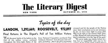
This resulted in Landon 55% and FDR 41%
The actual results:
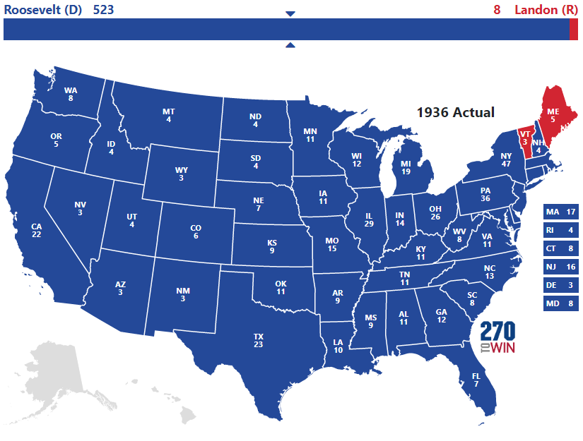
FDR 61% and Landon 37%.
So using error on the margin, the real result was FDR +24 and the poll had FDR -14, for a polling error of 38 points!
To benchmark, in 2020 – seen as a contemporary polling disaster – national polls had a Democratic bias of about 3 points and state polls had a Democratic bias of 4 points.
The question taken on by these article is the degree to which this polling error was a consequence of coverage error of non-response error.
Helpfully, Gallup was also polling during this time period (in a more systematic, but also flawed way). And in their poll they asked three key questions:
Do you own a phone/car?
Did you receive a Literary Digest ballot?
Did you send it in?
Remember that coverage error occurs when the people who are in the sampling frame have systematically different opinions than those people that are not in the sampling frame.
We can’t see the sampling frame directly here – but we know that Literary Digest used car registration lists and telephone books, which means that people without a car and phone were less likely to be covered by the poll.
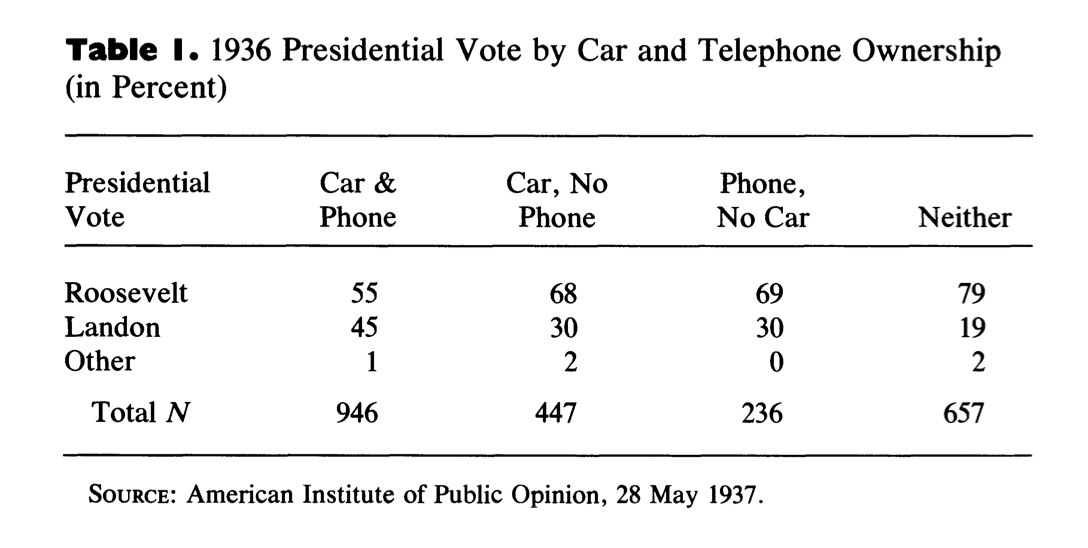
The first table looks at vote choice by these two variables. As the article discusses, because this poll was taken after the election, we expect that all of these numbers are probably a bit too high for Roosevelt. There is (or was, it’s probably less prevalent now) a consistent “winners effect” in post election polls where more people recall or report voting for the winning candidate than really did. Regardless, in every category Roosevelt, not Landon, is the preferred candidate. This is the first clue that it’s not just coverage error that caused the polling miss. For that to be the case there would have to be at least some group here who preferred Landon or Roosevelt. However, we do see that as someone is less likely to be in the sampling frame (not owning either a car or phone) they are more likely to support FDR. This is evidence that the people not in the samplign frame had different opinions (more pro FDR) than those in the sampling frame.
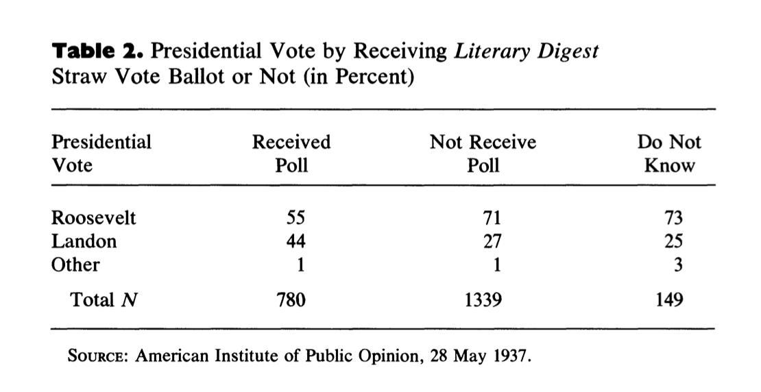
The second important question gets at the coverage issue in a more direct way. Because Literary Digest sent a postcard to nearly everyone in the sampling frame, simply asking if they got one is another look into the sampling frame. This might be a preferable question because we are asking people directly, but it might also suffer due to people forgetting whether they got a postcard or not.
This question shows relatively similar results. People who did not receive the LD poll (and therefore were not in the sampling frame) were more pro FDR than people who did receive the poll.
But these coverage issues alone are not enough to explain the polling miss. To do so we need to preview our next topic, which is non-response. Non-response bias occurs when their is correlation between responding to the poll and the question of interest (here vote choice). So in this third table we see, among those who received a ballot, whether there was a difference in opinion towards the candidates.
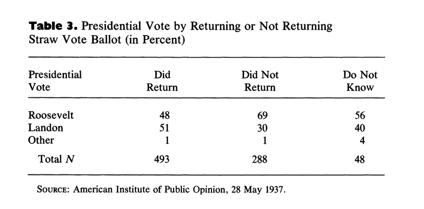
What we see is that the people who returend a ballot were far more likely to support Landon, and the people who did not return a ballot were far more likely to support Roosevelt. This indicates non-response bias was a significant contributor to the problem.
To sum this up: if everyone who was sent a ballot returned in the poll still would have been biased (that’s coverage error). And if everyone had been sent a ballot the poll still would have been biased (that’s non-response error). But both of these things happened at once, creating the huge error that brought down Literary Digest.
6.5 Questions
What is the margin of error for a poll of 100 people from a population of 500 people? What about from a population of 5000 people? Is applying a finite population correction in these cases a good idea?
I run a factory and produce 100 boxes of candy per day, each of which contains 1000 pieces. The overall variance in candy quality is 3, and the between box variance in candy quality is .5. I want to quality check the candy by eating 20 pieces of candy. Discuss how I might do this using simple random sampling and cluster sampling. What would be the key considerations I would need to take into account in order to make this decision?
-
I want to use stratified sampling to estimate support for higher education in the US
I propose splitting registered voters into strata based on their race. (Say 5 strata: white, black, hispanic, asian, and other). I want to sample 250 people from each strata. If I do this and take the mean of my sample’s opinions towards Trump, will I get an unbiased estimate of the population’s support for Trump?
Is race a good way to stratify the population for this question? What might be a better variable to stratify on?
Is is true or false that the 1936 Literary Digest poll would have gotten the right answer if they had sent their ballot to a representative sample of Americans?