8 Election Polling
Thus far we have mainly discussed polls that seek to measure the attributes of a known population. When we talked about Coverage Error we mainly discussed it as a function of a poorly specified sampling frame. For example: we may want to do a study of all students but we only have access to public school students.
Election polling represents a very different (and more challenging!) version of coverage error.
The fundamental challenge of election polling is that we are looking to poll a group of people who do not exist at the time of polling: voters.
We should indeed think of this as a problem of coverage. (Not that nonresponse isn’t also a problem for election polling, it definitely is). We have definied the samplign frame as a method that gives us a known and non-zero probability of accessing all members of the population. When our population is the group of people who will vote in an upcoming election that means developing a method that reliably captures the opinions of those who will vote (no undercoverage) while excluding those who will not vote (no ineligible units).
This is hard to do, and necessarily introduces fairly significant error into the polls – error that is absolutely not captured by the traditional margin of error.
But wait, is this really a problem? Like all other types of error, we both need to have the wrong people in our sampling frame, and the people who should and should not be in our sampling frame have to have different attitudes from one another. Put back into the language of election polling, for there to be error we need to have a poll that contains non-voters and those non-voters must have different opinions than the voters in the poll.
To help figure that out we need to know the differences between voters (eligible) and non-voters (ineligible) voters in a survey.
One source to help figure that out (and a source we are going to use a lot for this section) is the Cooperative Election Study. This is an academic study of registered voters. The CES is an RBS study, meaning that the sample was initially drawn from the voter file. Because we can link each respondent to the voter file, we can determine (after some time) whether that person voted or not. Therefore we have a variable in the survey that is not just whether the person plans to vote, it is a variable of whether they actually voted.
(This is not the only survey that does this. The other big one is the Current Population Study Voter Supplement.)
ces <- rio::import("https://github.com/marctrussler/IIS-Data/raw/refs/heads/main/CES_VV.Rds", trust=T)So our first goal is to see the degree to which people in this survey that are validated to vote have different opinions than those people that are not validated to vote.
We have a variable that tells us the proportion of the sample that voted in each of the election years:
ces |>
  group_by(year) |>
  summarise(mean(voted.general))
#> # A tibble: 7 × 2
#>    year `mean(voted.general)`
#>   <dbl>                 <dbl>
#> 1  2012                 0.667
#> 2  2014                 0.450
#> 3  2016                 0.555
#> 4  2018                 0.563
#> 5  2020                 0.643
#> 6  2022                 0.560
#> 7  2024                 0.607
I’ve also included a variable for people’s approval of the president. Let’s see if there is a difference in opinions for voters and non voters in each of these years.
ces|>
  group_by(year, voted.general) |>
  summarise(percent.dem = weighted.mean(approve.president, w=weight,na.rm=T)) |>
  pivot_wider(names_from = voted.general, values_from=percent.dem)
#> `summarise()` has grouped output by 'year'. You can
#> override using the `.groups` argument.
#> # A tibble: 7 × 3
#> # Groups:   year [7]
#>    year `FALSE` `TRUE`
#>   <dbl>   <dbl>  <dbl>
#> 1  2012   0.557  0.522
#> 2  2014   0.447  0.395
#> 3  2016   0.548  0.496
#> 4  2018   0.428  0.470
#> 5  2020   0.460  0.458
#> 6  2022   0.420  0.447
#> 7  2024   0.360  0.433
While it varies somewhat, in most years there is a good sized difference in the people who didn’t vote and the people who did. Some years there is little difference. The point is, we don’t know before the election if we are in a world like 2020 (virtually no difference) or a world like 2024 (7 points of difference).
Because of this, it’s important for us to identify voters and non-voters before the election in order to reduce the potential for coverage errors.
So how do we do that?
8.1 Identifying Likely Voters
To identify likely voters there are broadly two decisions to make: rely on self reports vs. a “covariate” approach; and to apply a deterministic or probablistic voter file filter. We will take each of these in turn.
8.1.1 Self reports
The first way we can think about identifying likely voters is via self-reported likelihood to vote. This is a simple and intuitive approach to this problem. Within our survey (probably of registered voters) we simply ask people if they are likely to vote to try to get at whether they will vote or not.
The CES asks such a question:
ces |>
  filter(year==2024) |>
  group_by(turnout.intent) |>
  summarise(n = n()) |>
  mutate(freq = n/sum(n))
#> # A tibble: 6 × 3
#>   turnout.intent                          n   freq
#>   <fct>                               <int>  <dbl>
#> 1 Yes, definitely                     38094 0.635
#> 2 Probably                             3677 0.0613
#> 3 I already voted (early or absentee)  9580 0.160
#> 4 I Plan to Vote Before November 5th   2600 0.0433
#> 5 No                                   3564 0.0594
#> 6 Undecided                            2485 0.0414
Here’s what that looked like in 2024. Around 64% of people said that they will definitely vote, and an additional 16% said that they had already voted.
The problem with this method is one of social desirability bias. As we have seen, a key source of measurement error occurs when people are motivated by norms to over-report something like voting.
What is nice about the CES is that (now, after the fact!) we can determine the degree of lying by seeing the actual probability that people in each of these groups ended up voting, or not.
ces |>
  filter(year==2024) |>
  group_by(turnout.intent) |>
  summarise(percent.voting = mean(voted.general,na.rm=T),
            n = n()) |>
  mutate(freq = n/sum(n))
#> # A tibble: 6 × 4
#>   turnout.intent                 percent.voting     n   freq
#>   <fct>                                   <dbl> <int>  <dbl>
#> 1 Yes, definitely                        0.679  38094 0.635
#> 2 Probably                               0.250   3677 0.0613
#> 3 I already voted (early or abs…         0.779   9580 0.160
#> 4 I Plan to Vote Before Novembe…         0.697   2600 0.0433
#> 5 No                                     0.0365  3564 0.0594
#> 6 Undecided                              0.0962  2485 0.0414
Of the people who say they will “definitely” vote, only 68% of those people actually vote. To be clear: some of the “non-voters” in this survey are people for whom CES couldn’t match them back to a voter file record (maybe they moved), so this is probably a slight under-estimate, but still this is a very high numbers of liars! Even for people who said that they already voted, just 78% of the people actually were verified to have voted.
So if we take those people at their word we will get some percentage of inelgible people in our survey: people who did not vote who we are calling voters.
While the problem is less severe, we also would have undercoverage if we completely disqualified those who said that they would not vote or where undecided. In those groups 4% and 10% voted, respectively.
So a single question does a just-ok job of predicting who will vote.
A more complex version of this process is to use a battery of questions to get at turnout. One traditionally used is the Perry-Gallup scale, developed by a Gallup researcher (Paul Perry) in the 1950s and 1960s. I’m sad that there wasn’t a guy named Perry Gallup. “Please, Mr. Gallup was my father. Call me Perry.”
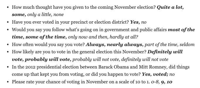
The 7 questions all try to tap the same underlying construct of “voting interest”. Having many questions and averaging them together will generally lead to a more reliable scale, however if there is a systematic bias (like desirability bias) that could still very well lead to a non-valid measure.
The respondents answer these questions and are given 1 point for selecting certain response categories (the ones bolded, above). Because young respondents were ineligible to vote in the past they are given bonus points. Ultimately each respondent is given a score between 0 and 7 which can then be used to identify voters and non-voters.
Does this scale do a better job of identifying voters and non-voters compared to a simple question? Pew has done a study where they applied this question in an RBS sample where they could late go back and determine whether people voted or not. (Same as what we just did with the CES.) Here are the results of that:

This gives us a bit more of a gradient (which will be helpful when we get to the next stage of actually applying these LV models) but largely has the same problems as what we saw above with the single question.
The people in the top category have an 83% chance of voting, so this does not reliably identify only voters. There is even bigger problems at the low end. At the bottom of the scale – people given a 0 and will almost certainly be screened out as non-voters – a full 11% of them voted. In total, for the 22% of voters who score between a 0 and 5, a pretty significant chunk voted. We also see that the scale very non-linearly identifies voters, even goign backwards at one point: voters with a score of 4 are less likely to vote than voters with a score of 3.
Relying on self reports is very simple and is very intuitive, but potentially introduces a lot of error by including ineligible voters and excluding eligibile voters.
8.1.2 Model based
The second way that we can determine voters and non-voters is a model based approach. Here what we want to do is to build a model of outcomes in a dataset where we have validated vote (like the CES). Then when we are in the present, we use the same variables for our respondents and the coefficients from the model to predict the probability that our respondents will vote.
Let’s pretend we are in 2024 at the time of interview and want to predict who is goign to vote. What we can do is answer the question: what predicted voting in 2020?
We know who voted in 2020, and we know things about those people. So let’s build a simple linear model in that year.
training <- ces |>
  filter(year==2020)

m1 <- lm(voted.general ~ sex + race + age4, data=training)
summary(m1)
#>
#> Call:
#> lm(formula = voted.general ~ sex + race + age4, data = training)
#>
#> Residuals:
#>     Min      1Q  Median      3Q     Max
#> -0.8509 -0.4603  0.1659  0.3751  0.7042
#>
#> Coefficients:
#>               Estimate Std. Error t value Pr(>|t|)
#> (Intercept)   0.314801   0.012114  25.988  < 2e-16 ***
#> sexFemale    -0.016878   0.004226  -3.994 6.51e-05 ***
#> raceBlack     0.003345   0.013027   0.257    0.797
#> raceHispanic -0.002106   0.012868  -0.164    0.870
#> raceOther     0.095931   0.015738   6.096 1.10e-09 ***
#> raceWhite     0.145469   0.011768  12.362  < 2e-16 ***
#> age430-44     0.164655   0.005599  29.410  < 2e-16 ***
#> age445-64     0.279105   0.006533  42.724  < 2e-16 ***
#> age465+       0.390670   0.005929  65.894  < 2e-16 ***
#> ---
#> Signif. codes:
#> 0 '***' 0.001 '**' 0.01 '*' 0.05 '.' 0.1 ' ' 1
#>
#> Residual standard error: 0.4564 on 48530 degrees of freedom
#>   (12461 observations deleted due to missingness)
#> Multiple R-squared:  0.1211, Adjusted R-squared:  0.121
#> F-statistic: 836.1 on 8 and 48530 DF,  p-value: < 2.2e-16
This is a really simple linear probability model that describes how each of these variables predict the probability of voting in 2020. Remember that in a regression model when we have a categorical variable we omit one category, and then the coefficients represent the change from that base category. Further, because our dependent variable is a binary variable (here a Boolean variable that R interprets as True=1 and False=0), these coefficients represent a change in the probability that someone is a voter.
So we see in this case that being a women (compared to being a man) reduces your probability of voting by 1.7%, bring Black (compared to Asian) rases your probability of voting by less than 1%, etc. The big action here in terms of impact is age, where the older you get the probability of voting raises substantially.
Regression can be used for description (what we are doing here), but it can also be used for prediction. In the 2024 data we have the exact same variables, and as such we can these coefficients and those variables to predict for each person what their probability of voting will be based off of their sex, race, and age.
test <- ces |>
  filter(year==2024)

test$vote.prob.lm <- predict(m1, newdata=test)
head(test$vote.prob.lm)
#> [1] 0.5803730        NA 0.8340624 0.2958169 0.8340624
#> [6] 0.6919380
This gives everyone in the survey a predicted probability of voting.
We can see that these probabilities are generated by the coefficients above. For example the average probability of voting for the different racial categories
test |>
  group_by(race) |>
  summarise(avg.prob = mean(vote.prob.lm, na.rm=T))
#> # A tibble: 5 × 2
#>   race     avg.prob
#>   <chr>       <dbl>
#> 1 Asian       0.466
#> 2 Black       0.536
#> 3 Hispanic    0.492
#> 4 Other       0.627
#> 5 White       0.711
Broadly representative of the coefficients we saw in the model above. (They don’t match the differences exactly because people’s scores are based on all their overlapping characteristics and the distribution of age and gender is not equal in all the races).
How well do these probabilities map onto actual voting. Again, because we have the actual validated vote data for these people we can look at this. To be clear, this is not something we would be able to do when we are actually building a likely voter model because the election would not have happened yet!
boxplot(test$vote.prob.lm ~ test$voted.general)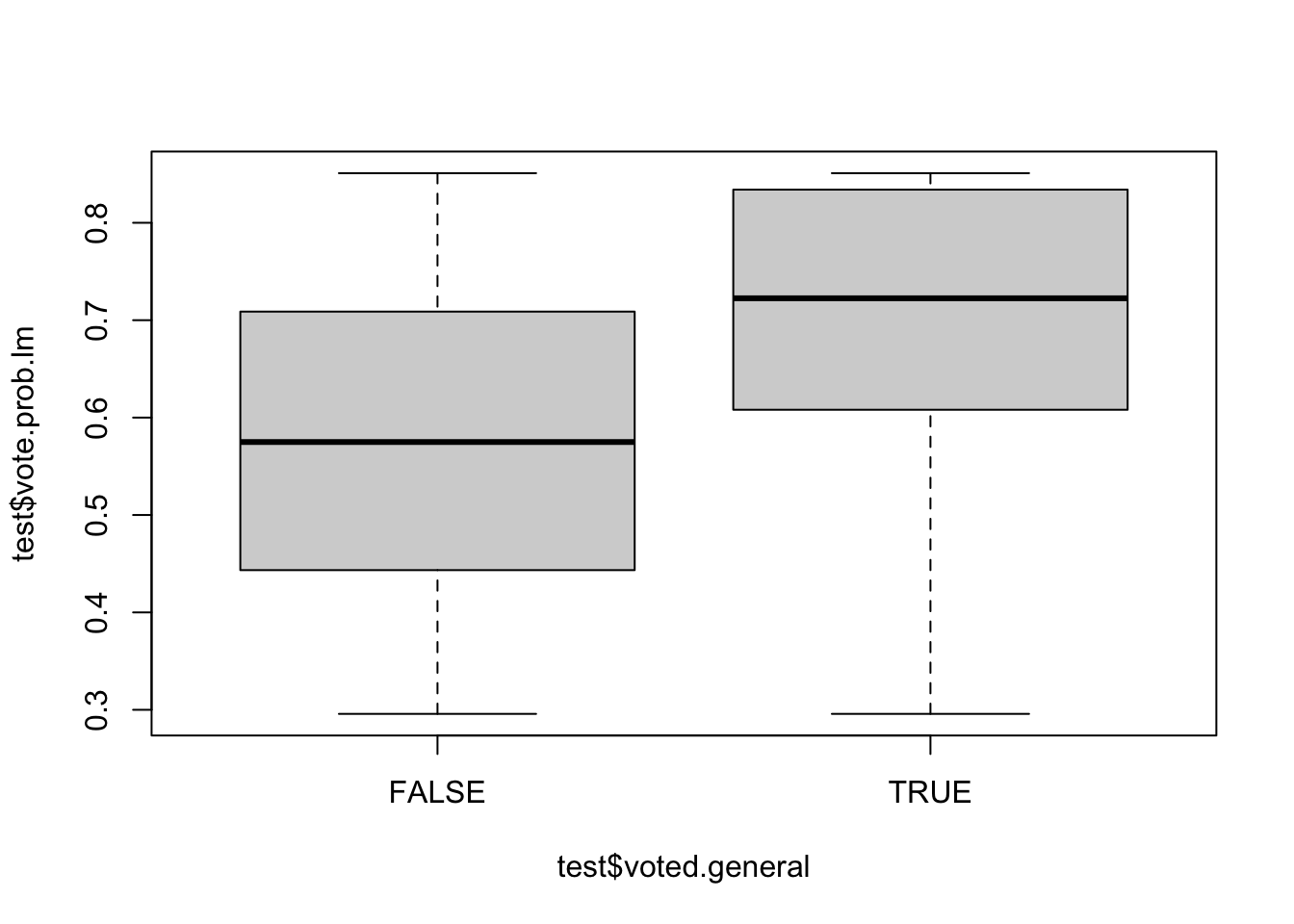
Very reasonably, the actual voters have much higher predicted vote probabilities than the actual non-voters.
What we are seeing here, in short, is that the relationship between these variables is stable across these two years. Older people voted more in 2020 and they did again in 2024. White people voted more in 2020 and they did again in 2020. But that’s the assumption we have to make in order for this modeling approach to work: that the relationship between these variables and voting is stable in the training and test data.
To sum up how good of a job we are doing, let’s take our probabilities and turn them into a binary predicted voter or predicted non-voter category. More about doing this below, and why this may not be the best case.
As we will see, the way we want to do this is to assign the tag of likely voter to all voters over a certain threshold. That threshold is determined by what we think the overall voting rate will be in the population. If 60% of people are going to vote in the population, than we should take the highest 60% of voting probabilities:
#The 40% quantile is the value that 60% of data is higher than
quantile(test$vote.prob.lm,.4, na.rm=T)
#>       40%
#> 0.6080475
#The fact that this is near 60% is a coincidence.

test |>
  mutate(likely.voter.lm = if_else(vote.prob.lm>.608,T,F)) -> test
How good of a job does that do?
test |>
  group_by(likely.voter.lm) |>
  summarise(vote.prob = mean(voted.general,na.rm=T))
#> # A tibble: 3 × 2
#>   likely.voter.lm vote.prob
#>   <lgl>               <dbl>
#> 1 FALSE               0.322
#> 2 TRUE                0.721
#> 3 NA                  0.693
28% of the people we predicted were voters did not vote, and 32% of the voters we predicted were not voters actually voted. So overall I would say that this model did ok.
Can we make this better? (Or potentially, make this even worse to see how it works?) Definitely!
The first thing that we want to do is to abandon the use of a simple linear model. We aren’t going to get into this in this class, but a simple linear probability model is great and intuitive, but has the bad feature of not being constrained in making predictions outside of the range of 0 and 1. That is bad! So we are going to switch to logistic regression. I don’t want you to worry about what this does, other than know that the predictions that it makes are bounded between 0 and 1.
So updating our code:
#Logit model on training data
m2 <- glm(voted.general ~ sex + race + age4, data=training, family="binomial")
summary(m2)
#>
#> Call:
#> glm(formula = voted.general ~ sex + race + age4, family = "binomial",
#>     data = training)
#>
#> Coefficients:
#>               Estimate Std. Error z value Pr(>|z|)
#> (Intercept)  -0.776864   0.055697 -13.948  < 2e-16 ***
#> sexFemale    -0.082663   0.020360  -4.060 4.91e-05 ***
#> raceBlack    -0.008629   0.059722  -0.144    0.885
#> raceHispanic -0.018038   0.058907  -0.306    0.759
#> raceOther     0.400061   0.072873   5.490 4.02e-08 ***
#> raceWhite     0.636104   0.053831  11.817  < 2e-16 ***
#> age430-44     0.677302   0.025204  26.873  < 2e-16 ***
#> age445-64     1.181114   0.030505  38.719  < 2e-16 ***
#> age465+       1.815602   0.030072  60.375  < 2e-16 ***
#> ---
#> Signif. codes:
#> 0 '***' 0.001 '**' 0.01 '*' 0.05 '.' 0.1 ' ' 1
#>
#> (Dispersion parameter for binomial family taken to be 1)
#>
#>     Null deviance: 64727  on 48538  degrees of freedom
#> Residual deviance: 58613  on 48530  degrees of freedom
#>   (12461 observations deleted due to missingness)
#> AIC: 58631
#>
#> Number of Fisher Scoring iterations: 4
#Predict in test data
test$vote.prob.log <- predict.glm(m2, newdata = test, type="response")
#Cut based on top 60%
test |>
  mutate(likely.voter.log =
           if_else(vote.prob.log>quantile(test$vote.prob.log,.4, na.rm=T),T,F)) -> test
#See Results
test |>
  group_by(likely.voter.log) |>
  summarise(vote.prob = mean(voted.general,na.rm=T))
#> # A tibble: 3 × 2
#>   likely.voter.log vote.prob
#>   <lgl>                <dbl>
#> 1 FALSE                0.373
#> 2 TRUE                 0.736
#> 3 NA                   0.693
This only made a marginal improvement, but is a much more sound way of doing it, particularly when we add more variables.
So let’s go about improving this.
First, let’s add additional election years. We have every election between 2012 and 2024. Should we add all of them? No, probably not. Again, our assumption here is that the variables that we choose have the same relationship predicting voting in our training and test data. Including midterm years would be assuming that the relationship between age and voting is equal across election types, and it probably isn’t!
Adding more general election years may help us get to a more general (and less 2020 specific) relationship between these variables which may lead to a better prediction in 2024. Alternatively, adding more years might make things worse because the relationships between the variables and voting may have changed! Let’s find out:
training <- ces |>
  filter(year %in% c(2012, 2016, 2020))
#Logit model on training data
m2 <- glm(voted.general ~ sex + race + age4, data=training, family="binomial")
summary(m2)
#>
#> Call:
#> glm(formula = voted.general ~ sex + race + age4, family = "binomial",
#>     data = training)
#>
#> Coefficients:
#>               Estimate Std. Error z value Pr(>|z|)
#> (Intercept)  -1.031121   0.034515 -29.874  < 2e-16 ***
#> sexFemale     0.003184   0.011710   0.272    0.786
#> raceBlack     0.411197   0.036353  11.311  < 2e-16 ***
#> raceHispanic  0.227183   0.036243   6.268 3.65e-10 ***
#> raceOther     0.609326   0.044478  13.699  < 2e-16 ***
#> raceWhite     0.820522   0.033423  24.550  < 2e-16 ***
#> age430-44     0.451829   0.015480  29.188  < 2e-16 ***
#> age445-64     0.917977   0.016929  54.224  < 2e-16 ***
#> age465+       1.623069   0.017558  92.441  < 2e-16 ***
#> ---
#> Signif. codes:
#> 0 '***' 0.001 '**' 0.01 '*' 0.05 '.' 0.1 ' ' 1
#>
#> (Dispersion parameter for binomial family taken to be 1)
#>
#>     Null deviance: 187555  on 138483  degrees of freedom
#> Residual deviance: 172846  on 138475  degrees of freedom
#>   (41651 observations deleted due to missingness)
#> AIC: 172864
#>
#> Number of Fisher Scoring iterations: 4
#Predict in test data
test$vote.prob.log <- predict.glm(m2, newdata = test, type="response")
#Cut based on top 60%
test |>
  mutate(likely.voter.log =
           if_else(vote.prob.log>quantile(test$vote.prob.log,.4, na.rm=T),T,F)) -> test
#See Results
test |>
  group_by(likely.voter.log) |>
  summarise(vote.prob = mean(voted.general,na.rm=T))
#> # A tibble: 3 × 2
#>   likely.voter.log vote.prob
#>   <lgl>                <dbl>
#> 1 FALSE                0.412
#> 2 TRUE                 0.730
#> 3 NA                   0.693
Well. This barely changed anything. Good to know I guess.
The other (probably more helpful) thing that we can do is to add more variables. Again, theoretically, having a better specified model can help us pick up the nuances that separate voters and non-voters. However, theoretically, doing so could make things worse! (You are seeing a theme). A risk here is overfitting a model that perfectly describes voting in a previous period to the detriment of being generalizable to future election years. Let’s find out by adding voter registration and education:
training <- ces |>
  filter(year %in% c(2012, 2016, 2020))
#Logit model on training data
m2 <- glm(voted.general ~ sex + race + age4 + registered + educ, data=training, family="binomial")
summary(m2)
#>
#> Call:
#> glm(formula = voted.general ~ sex + race + age4 + registered +
#>     educ, family = "binomial", data = training)
#>
#> Coefficients:
#>                  Estimate Std. Error z value Pr(>|z|)
#> (Intercept)      -5.35796    0.08546 -62.695  < 2e-16 ***
#> sexFemale        -0.07901    0.02206  -3.581 0.000342 ***
#> raceBlack        -0.01356    0.07111  -0.191 0.848813
#> raceHispanic      0.06570    0.07153   0.919 0.358321
#> raceOther         0.27424    0.08726   3.143 0.001673 **
#> raceWhite         0.43115    0.06695   6.440 1.19e-10 ***
#> age430-44         0.42153    0.02737  15.399  < 2e-16 ***
#> age445-64         0.82228    0.03005  27.367  < 2e-16 ***
#> age465+           1.88075    0.03496  53.800  < 2e-16 ***
#> registeredTRUE    7.00400    0.05313 131.821  < 2e-16 ***
#> educHs Or Less   -1.19873    0.03171 -37.800  < 2e-16 ***
#> educPostgrad      0.22913    0.04642   4.936 7.96e-07 ***
#> educSome College -0.58300    0.03116 -18.708  < 2e-16 ***
#> ---
#> Signif. codes:
#> 0 '***' 0.001 '**' 0.01 '*' 0.05 '.' 0.1 ' ' 1
#>
#> (Dispersion parameter for binomial family taken to be 1)
#>
#>     Null deviance: 187555  on 138483  degrees of freedom
#> Residual deviance:  61752  on 138471  degrees of freedom
#>   (41651 observations deleted due to missingness)
#> AIC: 61778
#>
#> Number of Fisher Scoring iterations: 7
#Predict in test data
test$vote.prob.log <- predict.glm(m2, newdata = test, type="response")
#Cut based on top 60%
test |>
  mutate(likely.voter.log =
           if_else(vote.prob.log>quantile(test$vote.prob.log,.4, na.rm=T),T,F)) -> test
#See Results
test |>
  group_by(likely.voter.log) |>
  summarise(vote.prob = mean(voted.general,na.rm=T))
#> # A tibble: 3 × 2
#>   likely.voter.log vote.prob
#>   <lgl>                <dbl>
#> 1 FALSE               0.0634
#> 2 TRUE                0.928
#> 3 NA                  0.693
We do a lot better! (The voter registration is helping a lot, to the point that we probably would just subset to registered voters before we even took this step). Now we are making many fewer errors. Just 8% of likely voters didn’t vote, and only 6% of unlikely voters actually voted. That’s good!
A lot of the variables we have used and discussed thus far are things we think are stable predictors of turnout. Old people always turn out more. Higher educated people always turn out more. But that leaves out something we might vaguely call enthusiasm. In every election there are groups of people, for reasons that are esoteric to that election, that are more likely to turn out to vote. Can we do something to incorporate something like that?
Well one of the reasons people may turn out is because of their partisanship. What if we include that in our model?
training <- ces |>
  filter(year %in% c(2012, 2016, 2020))
#Logit model on training data
m2 <- glm(voted.general ~ sex + race + age4 + registered + educ + pid5, data=training, family="binomial")
summary(m2)
#>
#> Call:
#> glm(formula = voted.general ~ sex + race + age4 + registered +
#>     educ + pid5, family = "binomial", data = training)
#>
#> Coefficients:
#>                     Estimate Std. Error z value Pr(>|z|)
#> (Intercept)         -5.18415    0.08898 -58.262  < 2e-16
#> sexFemale           -0.08238    0.02298  -3.585 0.000337
#> raceBlack           -0.10401    0.07416  -1.403 0.160745
#> raceHispanic         0.03085    0.07438   0.415 0.678332
#> raceOther            0.31379    0.09050   3.467 0.000526
#> raceWhite            0.42989    0.06976   6.163 7.15e-10
#> age430-44            0.43803    0.02866  15.281  < 2e-16
#> age445-64            0.80528    0.03133  25.707  < 2e-16
#> age465+              1.80406    0.03609  49.983  < 2e-16
#> registeredTRUE       7.00312    0.05384 130.075  < 2e-16
#> educHs Or Less      -1.13387    0.03284 -34.530  < 2e-16
#> educPostgrad         0.20469    0.04718   4.338 1.44e-05
#> educSome College    -0.55117    0.03202 -17.212  < 2e-16
#> pid5Independent     -0.67538    0.03244 -20.818  < 2e-16
#> pid5Lean Democrat   -0.04079    0.03811  -1.070 0.284489
#> pid5Lean Republican -0.10582    0.04347  -2.434 0.014913
#> pid5Republican      -0.03984    0.03078  -1.294 0.195598
#>
#> (Intercept)         ***
#> sexFemale           ***
#> raceBlack
#> raceHispanic
#> raceOther           ***
#> raceWhite           ***
#> age430-44           ***
#> age445-64           ***
#> age465+             ***
#> registeredTRUE      ***
#> educHs Or Less      ***
#> educPostgrad        ***
#> educSome College    ***
#> pid5Independent     ***
#> pid5Lean Democrat
#> pid5Lean Republican *
#> pid5Republican
#> ---
#> Signif. codes:
#> 0 '***' 0.001 '**' 0.01 '*' 0.05 '.' 0.1 ' ' 1
#>
#> (Dispersion parameter for binomial family taken to be 1)
#>
#>     Null deviance: 177724  on 132411  degrees of freedom
#> Residual deviance:  58002  on 132395  degrees of freedom
#>   (47723 observations deleted due to missingness)
#> AIC: 58036
#>
#> Number of Fisher Scoring iterations: 7
#Predict in test data
test$vote.prob.log <- predict.glm(m2, newdata = test, type="response")
#Cut based on top 60%
test |>
  mutate(likely.voter.log =
           if_else(vote.prob.log>quantile(test$vote.prob.log,.4, na.rm=T),T,F)) -> test
#See Results
test |>
  group_by(likely.voter.log) |>
  summarise(vote.prob = mean(voted.general,na.rm=T))
#> # A tibble: 3 × 2
#>   likely.voter.log vote.prob
#>   <lgl>                <dbl>
#> 1 FALSE               0.0761
#> 2 TRUE                0.934
#> 3 NA                  0.656
We actually do marginally better here, but I still don’t think that including partisanship is a good idea here. Remember the key assumption here is that the relationship between these variables and turning out will be even across elections. The whole point of elections is to reveal the partisanship of the electorate via voting. If we use a likely voter model that includes partisanship we are baking in an assumption that the partisanship of the previous electorate will equal the partisanship of the previous electorate. While it might be true, it doesn’t allow differential partisan enthusiasm to show up in a particular year’s polling.
(It’s probably the case that including partisanship resulted in a more accurate model because independents turn out at a significantly lower rate in every election.)
A better way to capture enthusiasm are “in-cycle measures”, the most commonly used is turnout in that year’s primary elections. We are seeing right now (I am writing this in 2025) an environment where Democrats are very fired up to vote. In every primary, special election, and the recent off-year elections in NJ and VA, we saw high democratic participation. In 2021, by contrast, Republicans were much more fired up and were more likely to turn out in these contests (and won the VA governorship and made the NJ race close).
We need a variable that would give Republicans a higher LV score in 2021 and Democrats a higher LV score in 2025. The way that we can do that is through including primary turnout in the model. Primary voters are fired up about politics and are more likely to vote in the general election. In one year that might mean Democrats, in another year that might mean Republicans. As long as we capture that relationship it doesn’t matter who shows up in the primary, they will get a higher LV score.
The nice thing about primary turnout is it is captured in the Vote File. We can build a model in the past seeing how verified primary vote affects verified general election vote:
training <- ces |>
  filter(year %in% c(2012, 2016, 2020))
#Logit model on training data
m2 <- glm(voted.general ~ sex + race + age4 + registered + educ + voted.primary, data=training, family="binomial")
summary(m2)
#>
#> Call:
#> glm(formula = voted.general ~ sex + race + age4 + registered +
#>     educ + voted.primary, family = "binomial", data = training)
#>
#> Coefficients:
#>                   Estimate Std. Error z value Pr(>|z|)
#> (Intercept)       -5.27654    0.08688 -60.731  < 2e-16 ***
#> sexFemale         -0.02225    0.02264  -0.983  0.32578
#> raceBlack          0.03326    0.07281   0.457  0.64782
#> raceHispanic       0.07548    0.07329   1.030  0.30311
#> raceOther          0.20853    0.08967   2.326  0.02004 *
#> raceWhite          0.37735    0.06860   5.501 3.79e-08 ***
#> age430-44          0.33483    0.02797  11.972  < 2e-16 ***
#> age445-64          0.66642    0.03073  21.683  < 2e-16 ***
#> age465+            1.44373    0.03608  40.012  < 2e-16 ***
#> registeredTRUE     6.53932    0.05304 123.288  < 2e-16 ***
#> educHs Or Less    -1.00888    0.03246 -31.081  < 2e-16 ***
#> educPostgrad       0.16727    0.04767   3.509  0.00045 ***
#> educSome College  -0.47586    0.03185 -14.940  < 2e-16 ***
#> voted.primaryTRUE  2.45580    0.04760  51.588  < 2e-16 ***
#> ---
#> Signif. codes:
#> 0 '***' 0.001 '**' 0.01 '*' 0.05 '.' 0.1 ' ' 1
#>
#> (Dispersion parameter for binomial family taken to be 1)
#>
#>     Null deviance: 187555  on 138483  degrees of freedom
#> Residual deviance:  56851  on 138470  degrees of freedom
#>   (41651 observations deleted due to missingness)
#> AIC: 56879
#>
#> Number of Fisher Scoring iterations: 7
Primary turnout is a significant, positive, predictor of turnout.
Let’s apply that to the 2024 data:
#Predict in test data
test$vote.prob.log <- predict.glm(m2, newdata = test, type="response")
#Cut based on top 60%
test |>
  mutate(likely.voter.log =
           if_else(vote.prob.log>quantile(test$vote.prob.log,.4, na.rm=T),T,F)) -> test
#See Results
test |>
  group_by(likely.voter.log) |>
  summarise(vote.prob = mean(voted.general,na.rm=T))
#> # A tibble: 3 × 2
#>   likely.voter.log vote.prob
#>   <lgl>                <dbl>
#> 1 FALSE               0.0585
#> 2 TRUE                0.931
#> 3 NA                  0.693
This leads to a small but meaninful improvement to our LV model.
8.1.3 Applying LV Scores
Once we have assigned a LV probability to each individual in the survey, how do we make use of it?
We should think about likely voter modelling as an additional step to weighting. Just like in weighting there is a difference in the distribution a variable (is a voter) in our sample and in the population. The population, in this case, is 100% voters! Our sample is not 100% voters. So we want to design weights that address this.
The simplest approach to this we saw above: to make the distribution of “is a voter” in our sample match the population some people should get a weight of 1 (is a voter) and some people should get a weight of 0 (is not a voter). This might be thought of as the “deterministic” method.
The goal here is to set a cut-off value that matches the predicted turnout of the election we are building our model for. Above, for a presidential election, we set the cut-off of 60%. Anyone with a score above that cut-off was determined to be a voter, anyone below it was determined to be a non-voter. We would then exclude the non-voters from our analysis. We can theoretically (and practically) think about this as multiplying the original weights by the outcome of the likely voter screen, such that the weight for non-voters goes to 0:
pewmethods::get_totals("vote.choice.president",test, "weight",na.rm=T)
#>   vote.choice.president   weight
#> 1            Democratic 43.14419
#> 2            Republican 47.13029
#> 3           Third Party  0.00000
#> 4                 Other  9.72552

test |>
  mutate(weight.lv = weight*likely.voter.log) -> test

pewmethods::get_totals("vote.choice.president",test, "weight.lv",na.rm=T)
#> Warning in make_weighted_crosstab(var, df, .x): Removed
#> 11606 rows containing missing values for weight.lv
#>   vote.choice.president weight.lv
#> 1            Democratic 46.904037
#> 2            Republican 46.787704
#> 3           Third Party  0.000000
#> 4                 Other  6.308259
This is a common and reaonable way to think about a likely voter screen. It’s particularly helpful if you have a very simple likely voter screen. Some polling firms very simply like deem anyone who says they are “very likely to vote” as their likely voters, and keeping only those people is the same sort of deterministic model being employed here.
The other way to apply these targets is to simply multiply together the original weights and the probability of voting. This takes a more nuanced view of voters where people more likely to be voters get a higher weight in the survey compared to people who have a low likelihood of voting.
To apply that process:
test |>
  mutate(weight.lv2 = weight*vote.prob.log) -> test

pewmethods::get_totals("vote.choice.president",test, "weight.lv",na.rm=T)
#> Warning in make_weighted_crosstab(var, df, .x): Removed
#> 11606 rows containing missing values for weight.lv
#>   vote.choice.president weight.lv
#> 1            Democratic 46.904037
#> 2            Republican 46.787704
#> 3           Third Party  0.000000
#> 4                 Other  6.308259
When we did normal rake weighting we made it so that the sum of the weights was equal to the sample size. Doing this is necessarily going to lead to a lower effective n. Comparing the deterministic and probabilitist methods of applying these scores we get new survey n’s of:
For both methods this reduces our \(n\) to around 24 thousand from an original sample size of 60,000.
This is also going to affect the variance of the weights.
pewmethods::calculate_deff(test$weight)
#> # A tibble: 1 × 6
#>       n mean_wt sd_wt  deff    ess   moe
#>   <int>   <dbl> <dbl> <dbl>  <dbl> <dbl>
#> 1 60000       1  1.46  3.13 19177. 0.708
pewmethods::calculate_deff(test$weight.lv)
#> # A tibble: 1 × 6
#>       n mean_wt sd_wt  deff    ess   moe
#>   <int>   <dbl> <dbl> <dbl>  <dbl> <dbl>
#> 1 27410   0.896  1.06  2.40 11401. 0.918
pewmethods::calculate_deff(test$weight.lv2)
#> # A tibble: 1 × 6
#>       n mean_wt sd_wt  deff    ess   moe
#>   <int>   <dbl> <dbl> <dbl>  <dbl> <dbl>
#> 1 45761   0.528 0.875  3.75 12199. 0.887
sm <- rio::import("https://github.com/marctrussler/IIS-Data/raw/refs/heads/main/NBCAug25Weighted.Rds", trust=T)8.2 Election Error Through the Lens of 2020
While 2016 gets the most attention for being a “bad year” for polls, it was actually 2020 that had the historic polling miss. This is the way it goes with election polls: if you get the winner right people care less about polling error, even if that error is larger than other years.
This particular election gives really good insight into where polling error can come from in an election poll, and what the particular contemporary challenges are in polling. It also shows the limitations to our analysis: the fundamental issue that we run into is that we cannot know the opinions of people who do not respond to our polls. Because of this fundamental fact we will not be able to form definitive conclusions about why the polls missed so badly in 2020.
8.2.1 (non) Accuracy of 2020 polls
When talking about the accuracy of election polls we are going to talk about the accruacy of the margin. That is the accuracy of the difference of the two candidates.
We can talk about this in two different ways.
The first is talking about the absolute error:
\[ |(Biden_{Poll} - Trump_{Poll}) - (Biden_{Vote} - Trump_{Vote}) | \]
What is the absolute value of the difference between the margin in the poll and the margin in the vote.
The real national margin in 2020 was 4.5 points for Biden. So a poll that had the national vote at Biden +6.5 would have an absolute error of 2 points, and a poll that had the national vote for Biden at +2.5 would also have an absolute error of 2 points. If these were the only two polls the average absolute error would be 2 points.
The other way to measure the error is the signed error: \[ (Biden_{Poll} - Trump_{Poll}) - (Biden_{Vote} - Trump_{Vote}) \]
This just removes the absolute value operator. So for this the same two polls: the poll that has Biden at +6.5 would have a signed error of +2 and the poll that has Biden at +2.5 would have a signed error of -2. If these were the only two polls than the average directional error would be 0.
We do really want to know both of these things. In a world with no signed error we would still want to know about the absolute error as a measure of the overall reliability (i.e. variance) of the polls.
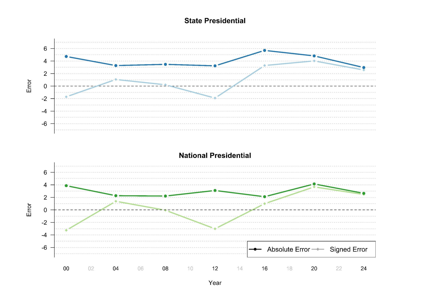
On these measures how did the 2020 polls do? This graph summarizes both for National polls in a comparative fashion:
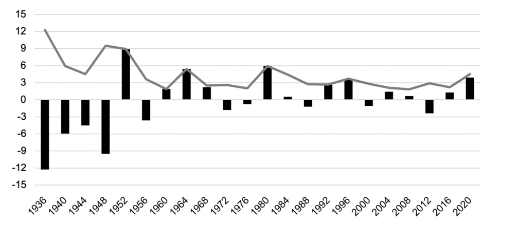
In this graph the gray line shows the average absolute error and the black bars show the signed error.
The average absolute error in 2020 was 4.5 points, which was larger than any error since the 1980 election. In comparison, the 2016 election had an absolute error of just 2.2 points, broadly in line with the previous 20 years of polling.
The average signed error in 2020 was 3.9 points, meaning that the average poll overstated Biden’s advantage by around 4 points. Given that this number is relatively close the the absolute error we can conclude that the error in the election was definitely systematically in Biden’s direction.
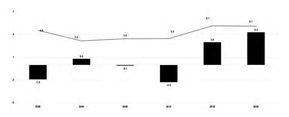
The news is even worse when we go to the state level. Here the average absolute error was just over 5 points. In comparison, that was actually the same amount of absolute error as in 2016.
However the signed error tells the full story here. While the absolute error was the same as 2016, the signed error increased to 4.3 percentage points. The state level polls were very biased towards Biden in 2020, and to a much larger degree than in 2016.
Critically: this average error gets worse when we switch our focus to statewide senatorial and gubernatorial polls. For those polls the average absolute error was 6.7 points and the signed error was 6 points in the Democratic direction. Significantly higher than the Presidential polls!
This leads to the first big conclusion about 2020 polling: this is not just a “Trump” phenomenon. Or, at least, this isn’t about how people discuss vote choice for Trump, specifically. We could imagine that a potential explanation for why the polls were biased against Trump is that people are reticent to admit that they are voting for Trump (or felt social desirability to say they were voting for Biden). But if that was true then we would only see this pro-Democratic effect in the Presidential race. The fact that the problem is worse in state level polling almost completely rules out social desirability as an explanation for the polling error.
8.2.2 Where did the polls miss
The other critical thing about the 2020 polling miss was that it was not even across all states. Here is what the signed polling error looked like across the country:
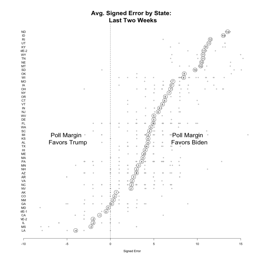
The biggest polling error in 2025 was in…. North Dakota?? That’s right. The three biggest places where the polls missed were North Dakota, Idaho, and Rhode Island.
Indeed, many of the most-error-prone states were heavily Republican states (excepting RI).
The swing state with he highest error was Wisconsin, but the rest of the swing states were pretty middle-of-the-pack for error. These misses obviously got the most attention (for good reason!) but they were not outliers in terms of the errors being made. (Nor were they made better by the huge amount of polling that went into them).
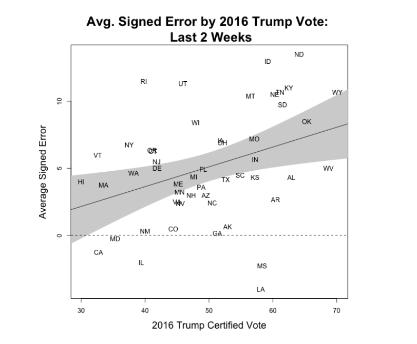
We can summarize these errors by looking across the 2016 results by state. While it’s not a deterministic relationship, in general the most pro-Biden errors were made in the states where Trump did the best. The states where Trump did the worst are the places where the polls were least likely to underestimate him.
8.2.3 Survey Mode
A potential explanation for higher survey error is what Bailey calls the new “Wild West” of polling, where an increasing number of firms are straying from traditional telephone based methodology. Might it be that these new methods are producing this error. Conversely: are outdated methods that rely on people pickup up their telephones causing the error.
To start out with, the distribution of survey modes in 2020 looked very different than in previous years.
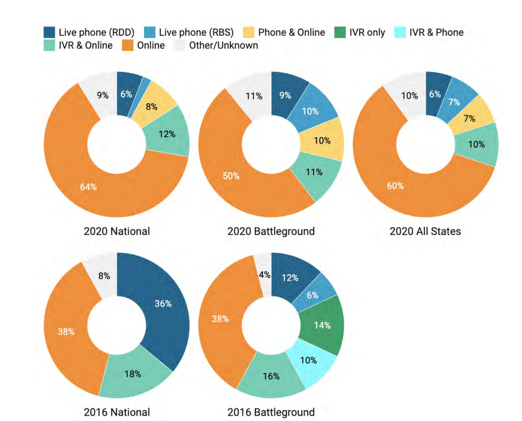
A way higher percentage of polls were online in 2020, and live phone RDD polls dropped to single digits. So there is at least the potential for this to be a major contributing factor.
In the AAPOR report, they simply break down the polling error based on what the mode of each poll was, the results for both absolute and signed error are presented in this figure:
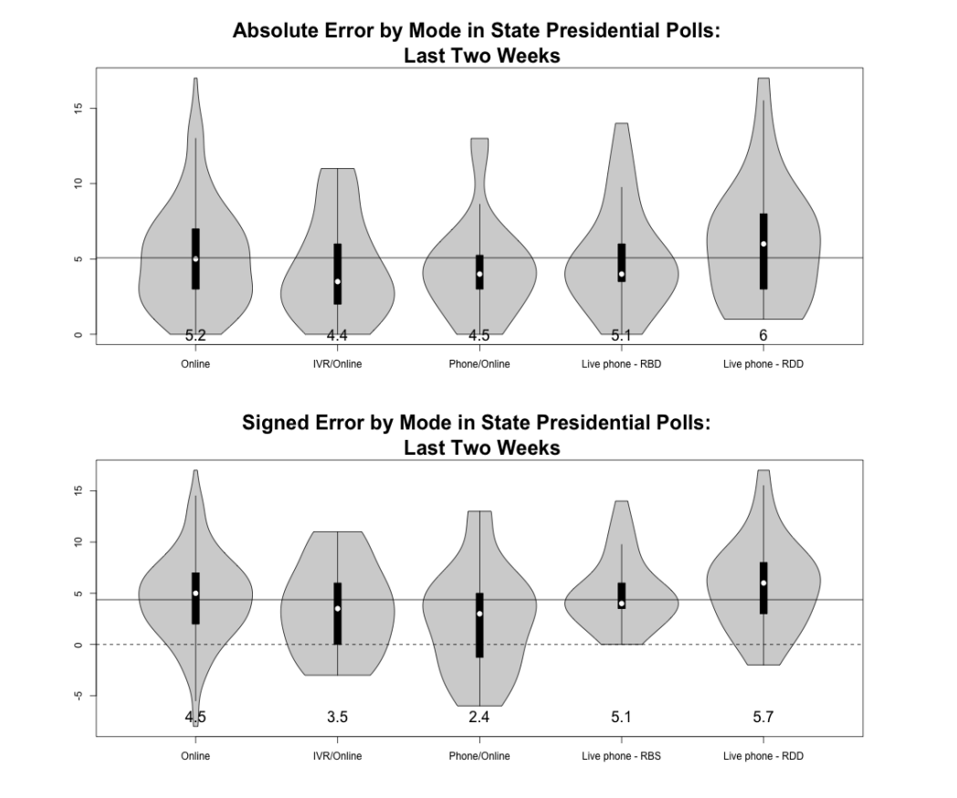
We can nibble around the edges here and figure out which one of these had higher error, but the truth is this just doesn’t seem to matter much.
There seems to be slightly lower error in polls that mix IVR (Interactive Voice Response) with online data collection. This is surprising! So called “robo polls” are generally thought to be the lowest quality of polls, but they ended up doing the best here.
In contrast the error seems to be slighty higher in polls that use telephone only methodology, with live caller RDD having the highest absolute and signed error. This is a bit surprising for RBS because this is thought to be the “gold standard” of election polling.
But overall, the message here is that survey mode just didn’t seem to matter very much in explaining the error. Remember this when peopel say “The polls missed because nobody answers their phones anymore!”
8.2.4 Explaining what happened
The report goes through several possible explanations of why the polls missed, thinking particularly about the pattern of the errors we saw above. I will summarize them here.
8.2.4.1 Late Deciders
In 2016 a major source of the error was late deciding voters moving decisively towards Trump. The conditions were ripe for such a thing in that year: both candidates were not very well liked so many voters were undecided. The news cycle moved in Trump’s favor in the close of the campaign and that shifted a fair chunk of voters towards him. This accounted for some of the polling error from polls conducted before that shfit took place.
The same dynamic does not seem to be in play in the 2020 polls.
First, there simply weren’t that many late deciding voters: only around 3-5% of voters were undecided in the polls approaching the election.
Second, the break in these voters was really inconsistent across surveys. Nationally they seemed to break towards Trump, but in many swing states they broke towards Biden.
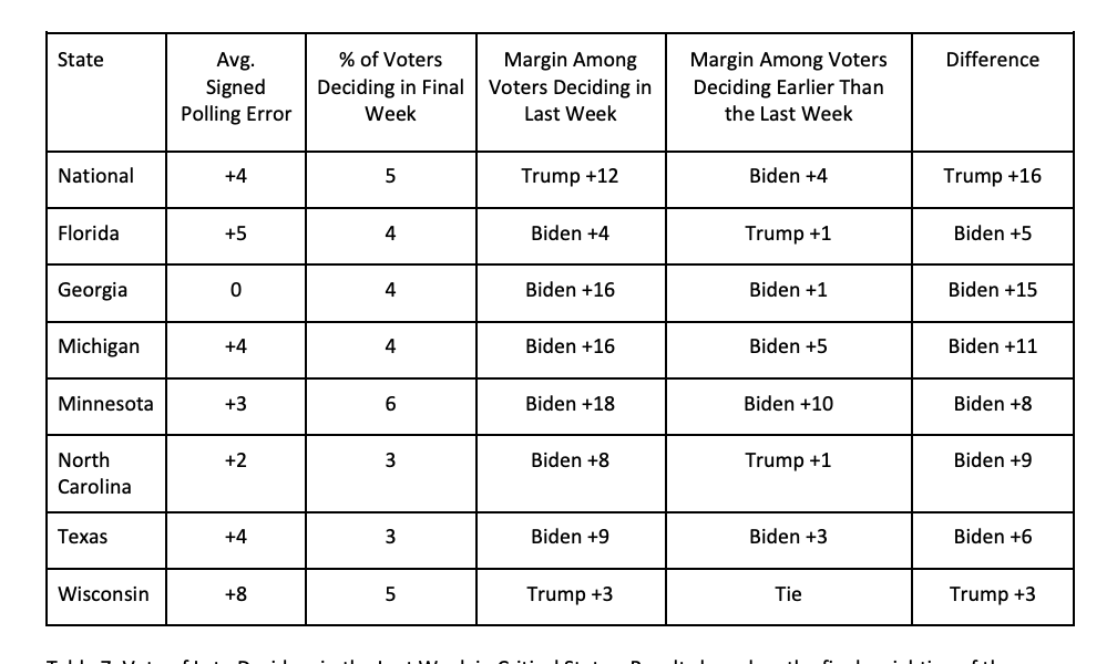
If you combine these things together it just cannot account for the persistent, large, polling error in a Biden direction.
8.2.4.2 Differences in self-reported intent to vote
Above when we discussed likely voter models we discussed models which used self-reports in some way to determine who is likely to vote. One possible source of error is if Democrats who stated they were likely to vote did not, or Republicans who stated they were unlikely to vote actually did. In other words, is there partisan differences in how stated intent to vote translated into actual turnout.
Using data like the CES above – where after the fact we use the voter file to determine who actually voted – we can look at that problem.
This table looks at this for one poll. First of all, their ineligible voter rate is very good! Around 90% of those who said they were going to vote actually did across all these polls and states.
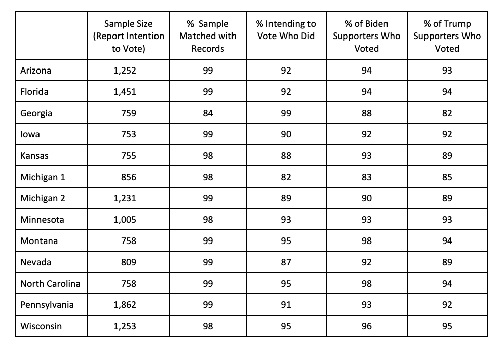
More importantly, there is virtually no difference between the percent of Biden supporters who actually voted and the percentage of Trump supporters who actually voted.
So this isn’t the answer either.
8.2.4.3 Errors related to “New” Voters
One particularly difficult thing to do in election polling is to account for the opinions of new voters. When we discussed likely voter modelling above, we discussed a lot about finding stable predictors of voting to use to estimate likely voters. New voters are (almost by definition) less likely to pass through these screens. We can think of this as an undercoverage problem – new voters are low propensity voters who have decided to turn out. If they have systematically different opinions then their exclusion can cause bias.
New voters were likely to be particularly problematic in 2020 because of the unprecedented turnout in the election. To get a lower bound of the potential number of new voters we can simply see how many more people voted in 2020 to 2016. If we assume that every 2016 voter voted in 2020 (probably wrong, back to this in a second), then the difference can be thought of as the percentage of new voters.
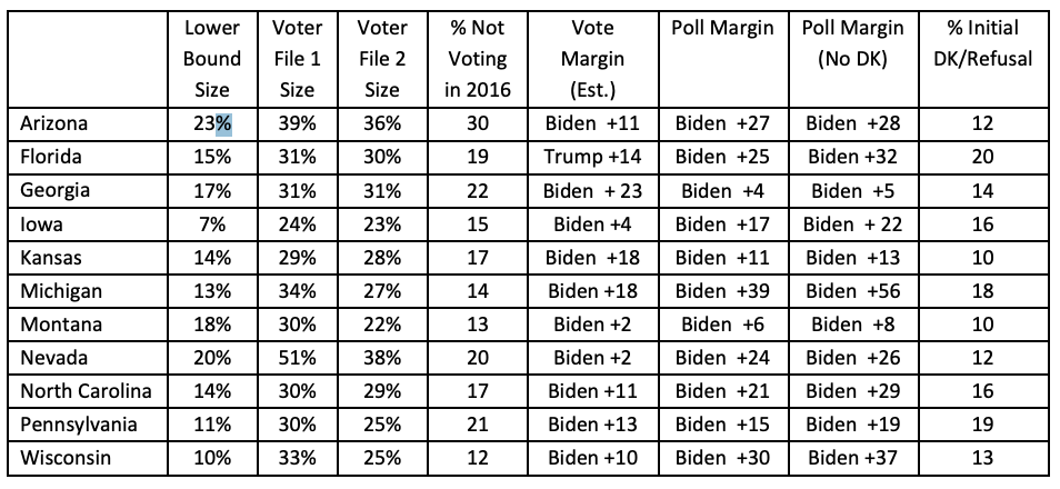
This is what is represented in the “Lower Bound” column. We see that the new voter rate was fairly high: around 15-20% in most of these states.
Now this is a lower bound because the assumption we made – everyone who voted in 2016 also voted in 2020 – is definitely wrong. Some of those people didn’t vote, and therefore the number of new voters is higher.
We can also attempt to use the voter file to determine how many new voters there are by looking at the percentage of 2020 voters who did not vote in 2016. Contrary to the lower bound, this number is almost certainly too high. Some of the trouble here is that people move and we are bad at matching people who have done so. Therefore some of the people we are calling “new” voters in this column are probably just “unmatched” voters.
Regardless, we can think of the true percentage of new voters to be somewhere between these two numbers.
In the column “% not voting in 2016” we get what was reported in the polls when we asked people if they had voted in 2015. These numbers are generally closer to the upper bound than the voter file estimate. This indicates that the polls were almost certainly systematically undercounting new voters. This is condition one for their to be a coverage problem!
But did the new voters we missed have different opinions compared to the new voters that we do have in our polls. Now, obviously, we can’t really know this! We didn’t interview the people we didn’t interview.
However, we can do some back of the envelope math to determine this. By making some assumptions (all Trump 2016 voters vote for Trump in 2020, all Clinton 2016 voters vote for Biden in 2020) we can back out from the results what has to be true of new voters in order to produce the change in the raw votes from one election to the next. That’s what’s in the “Vote Margin (Est.)” column.
What is critical is comparing that to the margin in the poll of the people who said they did not vote in 2016. Universally this number is more pro-Biden then the number we derive from the election results.
Put shorter: the polls missed a good chunk of new voters. The best evidence we have suggests that the new voters we do have in the polls were much more pro-Biden then the new voters we do not have in the polls.
Because of the “back of the envelope” nature of this analysis we cannot say anythign conclusive, but this is a really good candidate for where the polling error is coming from.
8.2.4.4 Error due to LV models, noncoverage, nonresponse
This is the most critical, but most subtle, area of possible error.
As I discussed above for Likely Voter models, we can think about the application of an LV model as a change to the weights. That’s true if we think about a deterministic model (where we would multiply LV’s weight by 1 and non-LV’s weight by 0) or a probabilistic model (where we multiply the original weights by the probability of voting). We end up with weights that are different from the original weights that will therefore imply a different distribution for demographic and political variables.
One way that we can determine the accuracy of our likely voter model is to adjust the weights to match the real election results and see the degree to which the weights for different categories change. If our original weights implied that the electorate would be 25% 18-29 year old’s, and after re-weighting to the actual results that group was now 20% of the electorate, it would indicate that our original LV model had too many people of that group.
The figure below does this for an RBS poll in PA:
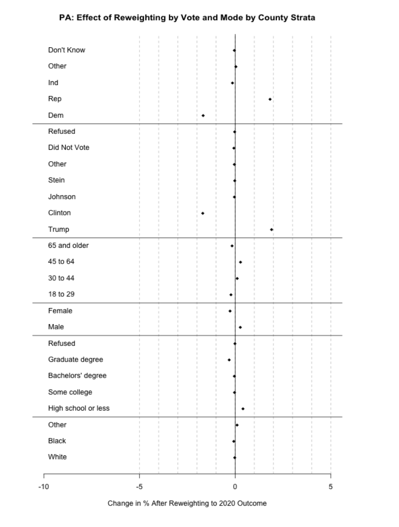
The upshot here is that the only variables that change their values are the political ones.
To put this in real terms: when it comes to age, gender, race, and education, the implied electorate in the original weights was dead on. It was not the case that pollsters assumed an electorate too non-white, or too-young. Those all seem to be correct.
What is wrong is the partisanship. When re-weighting the results it indicates that the original weights implied an electorate with too few Republicans and too many Democrats.
To make the original polls match the actual outcomes the Democrats in the sample would have had to be given less weight and the Republicans in the sample would have to be given more weight. The same could be done with 2016 vote: more weight to Trump voters, less weight to Clinton voters.
But here’s where it gets tricky: why is this pattern happening?
There are two possibilities, and unfortunately, we can’t really untangle them.
First: if we assume that we have a representive sample of Republicans, and a representative sample of Democrats, then the problem would be that we had too few Republicans and too many Democrats in our poll. We can broadly call this problem “between group missingness”. As we will see through the POQ paper next week, Republicans were systematically less likely to respond to polls in 2020, which increases the odds that what we are seeing here is a consequence of partisan non-response. But there is no if this is true because there is no real measure of the partisanship or past vote of the 2020 electorate.
Second: it might be that we had the correct number of Republicans and Democrats, but the Republicans and Democrats that we have in our poll are unrepresentative of all Republicans and Democrats. For example: the Republicans we have in our poll may be, on balance, more likely to support Joe Biden (Never Trumpers), while the Republicans who do not respond to our poll are more likely to support Trump (MAGA). This would result in it seeming like we have “too few” Republicans, when in reality we just have a group of Republicans who are not supportive of Trump in a representative way.
If the true problem is this last problem (and, to be honest, I think it is) then weighting to a correct measure of partisanship or to past vote will not reduce the errors of the polls.
8.2.5 Updating to 2024
The 2024 version of this report came out literally one week ago. (As of first writing of this, in November 2025).
I don’t have time to fully go through this new report, but we can quickly glance at the executive summary to see if this problem is continuing, and what the new theories are on what went wrong.
The overall topline numbers show that polling error improved in 2024. Both in terms of absolute and signed error, and in both national and state polls, the polling was better in 2024 than in 2020.
Generally they find that “higher volume firms, those weighting on partisan self-identification, those using detailed likely voter models, and Republican-affiliated pollsters were slightly more accurate.”
In general (from my brief reading of this report) the gains from 2020 come from two places: (1) more consistently weighting to past vote/partisanship to account for non-response (though this can go wrong); and (2) turnout overall was lower so the problem with “new’ voters was proportionally smaller.