7 For/If
Updated for S2026? No.
This week we are going to work with the ACS county data once again.
acs <- rio::import("https://github.com/marctrussler/IDS-Data/raw/main/ACSCountyData.csv")One of the most flexible tools in all coding languages is for() loops. In short: for() loops allow us to repeat the same code many, many, times. There are a couple of reasons why this is helpful. For this class the primary use case are situations where we need to perform the same observation on different clusters in the data. Below, for example, we want to perform the same operation on all of the counties in one state, and then move to the next state etc.
The other use case is when we want to use R to simulate probability. This won’t come up a lot in this class but is a big component of PSCI 1801, the followup to this class.
Previously we learned about how we can use the square brackets to give us conditional means.
For example we can easily get the mean population for all counties:
mean(acs$population)
#> [1] 102769.9
And if we want the mean population for just the counties in Alabama:
mean(acs$population[acs$state.abbr=="AL"])
#> [1] 72607.16
OK, but what if we wanted to do the same thing for all 50 states?
We could think about brute forcing it, subbing in the right two letter abbreviation and repeating the code 50 times:
mean(acs$population[acs$state.abbr=="AK"])
#> [1] 25466.07
mean(acs$population[acs$state.abbr=="AZ"])
#> [1] 463112.3
mean(acs$population[acs$state.abbr=="AR"])
#> [1] 39875.61
mean(acs$population[acs$state.abbr=="CA"])
#> [1] 674978.6
#
#
#
#
mean(acs$population[acs$state.abbr=="WI"])
#> [1] 80255.47
mean(acs$population[acs$state.abbr=="WY"])
#> [1] 25297.22
This is unwieldy! And I didn’t even do all of the states!
But notice something about the above block of code: most of the command on each line is exactly the same. All that we are changing in every line is what is in the quotations. WE are going from AL, to AL, to AZ…. all the way to WY.
So all we need is a method that allows us to run mean(acs$population[acs$state.abbr=="XX"]) 50 times, each time through changing XX to the next two-letter stabe abbreviation.
The way that we will accomplish this is with a for() loop.
Here is the basic setup for a for() loop:
for(i in 1:3){
  #CODE HERE
}
We can look at the for loop as having two parts. Everything from the start to the opening squiggly bracket are the instructions for the loop. It basically tells the loop how many times to repeat the same thing. “i” in this case is the variable that is going to change its value each time through the loop. Having this variable is what allows the loop to do something slightly different each time through the loop. The second part is whatever you put in between the squiggly brackets. This is the code that will be repeated again, and again the specified number of times.
Let’s put a simple bit of code in the loop to see how these work. I’m just going to put the command print(i) in the loop so that all the loop does is print the current value of i.
for(i in 1:3){
  print(i)
}
#> [1] 1
#> [1] 2
#> [1] 3
What a loop does is the following: on the first time through the loop it sets our variable (i) to the number 1. Literally. Anywhere we have the variable i, R will replace it with the integer 1. Once all the code has been executed and R reaches the closing squiggly bracket it goes back up the start. Now it will set i equal to 2. Anywhere in our code where there is currently the variable “i”, R will literally treat this as the integer 2. After it reaches the end of the code again, it will go back to the beginning and run the code again, this time making “i” equal to 3.
So the result of running this code is to simply print out the numbers 1, then 2, then 3.
To make this crystal clear, here is what code is literally being executed by R here. It is just the print command 3 times, the first time changing the variable i to the integer 1, the second time changing it to 2, and the third time changing it to 3.
Let’s take a second to think through the options at the start of this loop; everything that is contained in the opening parentheses.
Right now it says for(i in 1:3). This is saying: the variable that’s going to change everytime through the loop is called “i”, and the things we want to change it to is the sequence of numbers 1, 2, and then 3. Each of these things is customizable.
First, there is nothing special about “i”. We can name the variable that changes everytime through the script to anything we want.
So, for example, we can edit this same code to be for(batman in 1:3), and have the variable be called batman. And if we run this we get the exact same result.
for(batman in 1:3){
  print(batman)
}
#> [1] 1
#> [1] 2
#> [1] 3
This being said, it is convention to use the letter “i” as the indexing variable in a for loop. This is true across coding platforms so it’s a good idea to just use that.
Second, we can put any sort of vector into the second part. We can make it longer, for example, by running from 1 to 50.
for(i in 1:50){
  print(i)
}
#> [1] 1
#> [1] 2
#> [1] 3
#> [1] 4
#> [1] 5
#> [1] 6
#> [1] 7
#> [1] 8
#> [1] 9
#> [1] 10
#> [1] 11
#> [1] 12
#> [1] 13
#> [1] 14
#> [1] 15
#> [1] 16
#> [1] 17
#> [1] 18
#> [1] 19
#> [1] 20
#> [1] 21
#> [1] 22
#> [1] 23
#> [1] 24
#> [1] 25
#> [1] 26
#> [1] 27
#> [1] 28
#> [1] 29
#> [1] 30
#> [1] 31
#> [1] 32
#> [1] 33
#> [1] 34
#> [1] 35
#> [1] 36
#> [1] 37
#> [1] 38
#> [1] 39
#> [1] 40
#> [1] 41
#> [1] 42
#> [1] 43
#> [1] 44
#> [1] 45
#> [1] 46
#> [1] 47
#> [1] 48
#> [1] 49
#> [1] 50
We could also use the concatenate (or c() function) to give it a sequence of numbers to loop through. So here the first time through the loop i will be set equal to 2, the second time through it will be set equal to 15, and the third time through it will be set equal to 45.
Before you run this code, think: what code would the following produce?
Now let’s use our knowledge of for() loops to complete the task we set out: calculating the mean population for the counties in every state.
Let’s start by simply dropping in our code that we already have into our loop function.
for(i in 1:3){
  mean(acs$population[acs$state.abbr=="AL"])
}
Now, our target here is to change the state from AL, to AZ, to AR etc. each time through the loop. How can we use the functionality of loops, where R will sequentially change the variable i from 1, to 2, to 3 etc to accomplish that.
The way we are going to do that is to first create and save a vector of all the state abbreviations.
Using the unique() command, I can create a vector of all the state abbreviations. If we look at this, we now have a vector of all the possible state abbreviations. AL is first, AK is second, AZ is third.
states <- unique(acs$state.abbr)
states
#>  [1] "AL" "AK" "AZ" "AR" "CA" "CO" "CT" "DE" "DC" "FL" "GA"
#> [12] "HI" "ID" "IL" "IN" "IA" "KS" "KY" "LA" "ME" "MD" "MA"
#> [23] "MI" "MN" "MS" "MO" "MT" "NE" "NV" "NH" "NJ" "NM" "NY"
#> [34] "NC" "ND" "OH" "OK" "OR" "PA" "RI" "SC" "SD" "TN" "TX"
#> [45] "UT" "VT" "VA" "WA" "WV" "WI" "WY"
Remember that by using square brackets we can select a certain value out of a vector. So the first entry in states is AL, the 13th entry in states is ID, and the 27th entry in states is Montana.
states[1]
#> [1] "AL"
states[13]
#> [1] "ID"
states[27]
#> [1] "MT"
So instead of subsetting to a particular two letter abbreviation, now we can insert this vector and have the loop sequentially select each of the items in it each time through the loop. The first state, the second state etc
for(i in 1:3){
  mean(acs$population[acs$state.abbr==states[i] ])
}
So instead of acs$state.abbr=="AL", we will have acs$state.abbr==states[i].
Again, let’s think about what R is going to do in this code. The first time through the loop it will change i to the integer 1, then the integer 2, then the integer 3. This successfully accomplishes what we want, successively subsetting to each state, one-by-one.
So here we are calculating the mean county population for the first state (AL), then the second state (AK), then the third state (AZ)
#What it will literally do
mean(acs$population[acs$state.abbr==states[1]])
#> [1] 72607.16
mean(acs$population[acs$state.abbr==states[2]])
#> [1] 25466.07
mean(acs$population[acs$state.abbr==states[3]])
#> [1] 463112.3
But hold on, right now we are only going from 1 to 3, but there are 50 states + DC. So we need to edit the code to go from 1:51. Sequentially changing the variable i to 1, then to 2, then to 3, then to 4, all the way up to i equaling 51.
The easiest way to do this is to just write in 1:51 instead of 1:3. This will work fine, but I would encourage one slightly better coding practice here. What if,in the future, you decide that you don’t want this answer for DC, so now the vector “states” is only 50 items long? In that case we’d have to go in and change it from 1:51 to 1:50. Or, maybe, in the future we add data on Puerto Rico so now we have to remember to change this loop to 1:52.
for(i in 1:51){
  mean(acs$population[acs$state.abbr==states[i] ])
}
A better thing to do is to set the end point of the loop to be the length of the vector states, regardless of what the length is. So i’m going to edit my loop to run from 1:length(states). If we highlight the length(states) we see that rigt now it is 51, but if we ever change it in the future, our code will still work.
Now let’s run it and see what happens: nothing!
What’s happened here. R, in fact, did run the command in the brackets 51 times, each time changing i from 1 to 2 to 3, effectively looping over the 50 states + DC.
But unless we explicitly tell R to save the results of what it is doing, it will do all of this in the background when running code inside a loop.
So the last step in this process is to create an empty vector to store the results. We need to create a vector of NAs that is the same length as states. So i’m going to create the vector state.pop.means that is a vector that repeats NA for the same length as the “states” vector.
And each time through the loop we will assign the result of what we are doing to this new vector.
state.pop.means <- rep(NA, length(states))

#Ok let's try this:

for(i in 1:length(states)){
state.pop.means <- mean(acs$population[acs$state.abbr==states[i] ])
}
state.pop.means
#> [1] 25297.22
OK! Let’s give this a shot. Huh. Well that didn’t work. We were expecting to get 51 state means in this vector, but instead we got just one. Why did that happen?
Well, the first time through the loop we told R: assign the mean of alabama to the object “state.pop.means”, and it did. Then we said, OK, nevermind, assign the mean of alaska to “state.pop.means”. Then we said, OK, nevermind, assign the mean of arkansas to “state.pop.means”. So this 25297 is just the last mean we calculated (the average population of counties in Wyoming).
The last step here is to tell R to save the results in the right “slot” of state.pop.means. We do this by using our variable i to index the results column as well. Here’s what that looks like. So each time through the loop we are saving the results to the first slot in state.pop.means, and then the next time in the second slot of state.pop.means etc. And running the command we see that we did indeed get an answer for every state!
state.pop.means <- rep(NA, length(states))

for(i in 1:length(states)){
  state.pop.means[i] <- mean(acs$population[acs$state.abbr==states[i] ])
}

cbind(states,state.pop.means)
#>       states state.pop.means
#>  [1,] "AL"   "72607.1641791045"
#>  [2,] "AK"   "25466.0689655172"
#>  [3,] "AZ"   "463112.333333333"
#>  [4,] "AR"   "39875.6133333333"
#>  [5,] "CA"   "674978.620689655"
#>  [6,] "CO"   "86424.078125"
#>  [7,] "CT"   "447688"
#>  [8,] "DE"   "316498.333333333"
#>  [9,] "DC"   "684498"
#> [10,] "FL"   "307434.910447761"
#> [11,] "GA"   "64764.0503144654"
#> [12,] "HI"   "284405.8"
#> [13,] "ID"   "38359.2954545455"
#> [14,] "IL"   "125700.950980392"
#> [15,] "IN"   "72145.9347826087"
#> [16,] "IA"   "31641.404040404"
#> [17,] "KS"   "27702.6285714286"
#> [18,] "KY"   "37001.7"
#> [19,] "LA"   "72869"
#> [20,] "ME"   "83300.8125"
#> [21,] "MD"   "250143.125"
#> [22,] "MA"   "487870.928571429"
#> [23,] "MI"   "119969.734939759"
#> [24,] "MN"   "63532.8505747126"
#> [25,] "MS"   "36448.3170731707"
#> [26,] "MO"   "52957.0608695652"
#> [27,] "MT"   "18602.3571428571"
#> [28,] "NE"   "20481.2903225806"
#> [29,] "NV"   "171932.294117647"
#> [30,] "NH"   "134362.2"
#> [31,] "NJ"   "422945"
#> [32,] "NM"   "63407.0909090909"
#> [33,] "NY"   "316426.661290323"
#> [34,] "NC"   "101556.24"
#> [35,] "ND"   "14192.4716981132"
#> [36,] "OH"   "132294.079545455"
#> [37,] "OK"   "50884.8961038961"
#> [38,] "OR"   "113387.305555556"
#> [39,] "PA"   "190913.149253731"
#> [40,] "RI"   "211322.2"
#> [41,] "SC"   "107737.5"
#> [42,] "SD"   "13095.2878787879"
#> [43,] "TN"   "70011.4631578947"
#> [44,] "TX"   "109784.232283465"
#> [45,] "UT"   "105012.068965517"
#> [46,] "VT"   "44641.2142857143"
#> [47,] "VA"   "63261.4586466165"
#> [48,] "WA"   "187034.256410256"
#> [49,] "WV"   "33255.5272727273"
#> [50,] "WI"   "80255.4722222222"
#> [51,] "WY"   "25297.2173913043"
Again, we can always take the command out of the loop, literally enter the integers, and get a sense of what R is doing. I do this all the time! Here we see clearly what is happening.
state.pop.means[1] <- mean(acs$population[acs$state.abbr==states[1] ])
state.pop.means[2] <- mean(acs$population[acs$state.abbr==states[2] ])
state.pop.means[3] <- mean(acs$population[acs$state.abbr==states[3] ])
state.pop.means[4] <- mean(acs$population[acs$state.abbr==states[4] ])
state.pop.means[5] <- mean(acs$population[acs$state.abbr==states[5] ])
state.pop.means[6] <- mean(acs$population[acs$state.abbr==states[6] ])
state.pop.means[7] <- mean(acs$population[acs$state.abbr==states[7] ])
state.pop.means[8] <- mean(acs$population[acs$state.abbr==states[8] ])
state.pop.means[9] <- mean(acs$population[acs$state.abbr==states[9] ])
state.pop.means[10] <- mean(acs$population[acs$state.abbr==states[10] ])
state.pop.means[11] <- mean(acs$population[acs$state.abbr==states[11] ])
state.pop.means[12] <- mean(acs$population[acs$state.abbr==states[12] ])
#
#
state.pop.means[51] <- mean(acs$population[acs$state.abbr==states[51] ])
Each time through the loop our variable i gets changed to a new value. The first time through the loop changing i to the integer 1 accomplishes two tasks. First, it tells R which slot in the empty vector “state.pop.means” to save the answer. Second, it tells which entry in the vector “states” to access in order to subset our data.
So always try to remember that nothing more complicated than this is happening inside of a loop. And you can always just enter the integers yourself to get a sense of what is going on.
7.0.1 Example
Let’s create a new variable that splits counties into population density deciles. For each of those deciles, we want to calculate the median unemployment rate.
acs$pop.density.deciles <- dplyr::ntile(acs$population.density, 10)How does this decile function work?
table(acs$pop.density.deciles)
#>
#>   1   2   3   4   5   6   7   8   9  10
#> 315 315 314 314 314 314 314 314 314 314
mean(acs$population.density[acs$pop.density.deciles==1])
#> [1] 2.10158
mean(acs$population.density[acs$pop.density.deciles==10])
#> [1] 2108.274
Note that if we just wanted to visualize this we don’t need to go and calculate every median. The boxplot function does this for us. In the boxplot function if we have a continuous variable (like population density) and want to look at it over multiple discrete categories (like the deciles we just calculated) we can do:
boxplot(acs$population.density ~ acs$pop.density.deciles)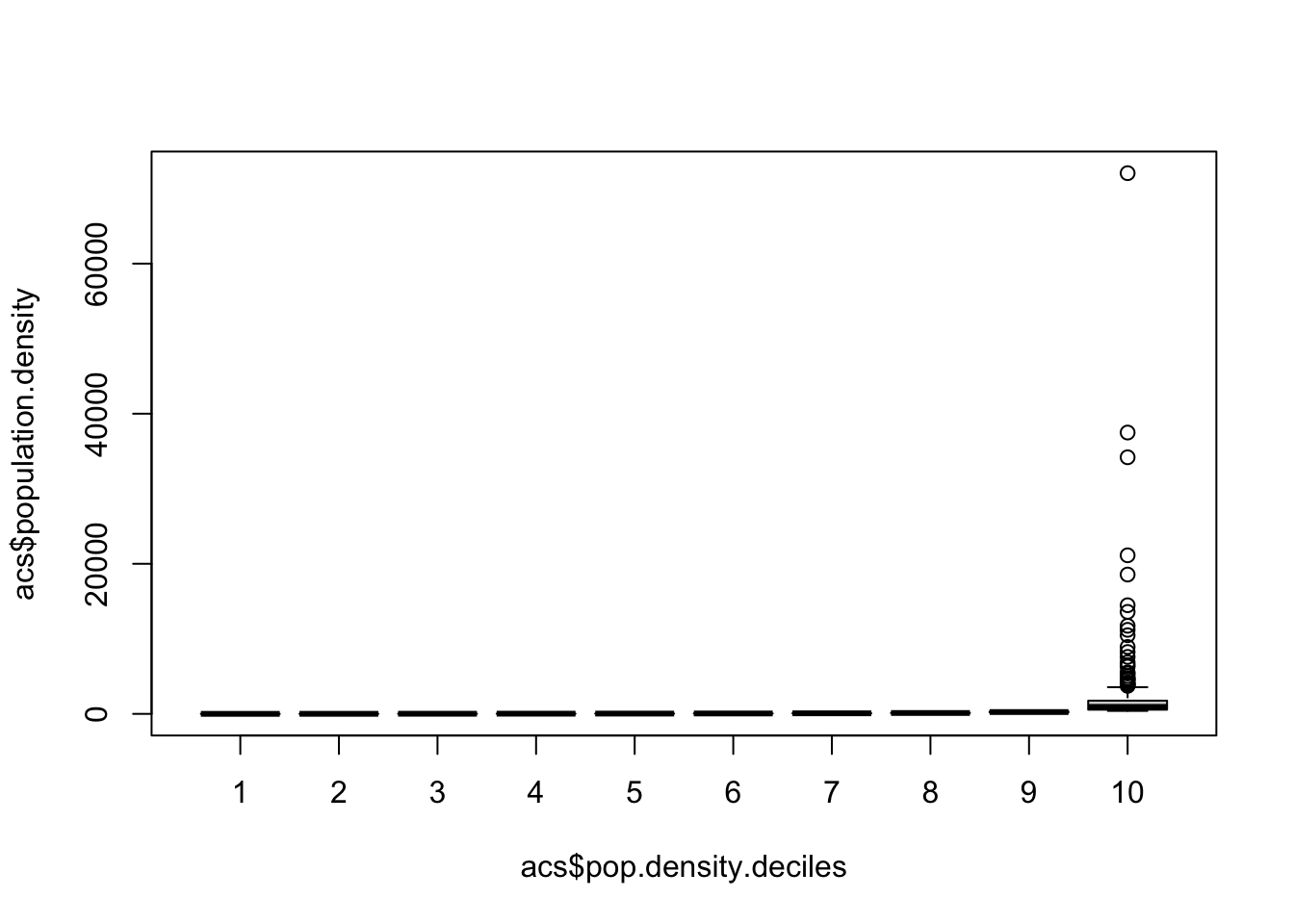
Note that with boxplot if you have some extreme outliers it will show them as additional points. Here there are 20 or so counties that have a population density far outside the normal range. We can just remove them to better visualize the data
boxplot(acs$population.density ~ acs$pop.density.deciles, outline=F)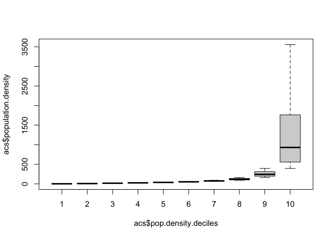
Even still, the 10% of counties that are the largest are so big that it makes this chart pretty useless.
Let’s recover the median population density for each of these deciles.
dec <-seq(1,10,1)

median.pop <- rep(NA, length(dec))

for(i in 1: length(dec)){
  median.pop[i] <- median(acs$population.density[acs$pop.density.deciles==dec[i]])
}

cbind(dec,median.pop)
#>       dec median.pop
#>  [1,]   1   2.063226
#>  [2,]   2   7.611136
#>  [3,]   3  16.748455
#>  [4,]   4  26.387725
#>  [5,]   5  37.837605
#>  [6,]   6  52.352135
#>  [7,]   7  75.421505
#>  [8,]   8 117.046250
#>  [9,]   9 244.075750
#> [10,]  10 930.521250
7.0.2 Example 2: Probability
If you go on to take PSCI1801: Statistical Methods in the fall we will use loops a lot in the study of probability.
Let’s say we want to know the odds of getting 0 heads when we flip a coin 7 times. There is a way to calculate this mathematically, but a way to think about probability is simply finding the relative frequency that an event occurs when we repeat an exercise a large number of times. We can get at this in R by literally (well, virtually, through code) flipping 7 coins a large number of times and seeing how often we get 0 heads.
Before we do this a large number of times, let’s create the code to do it once.
First, let’s create an object called coin that is just a vector with 0 and 1 in it. We’ll define 0 as tails, and 1 as heads.
coin <- c(0,1)The sample() command take a random sample from an object a specific number of times. Here we are going to sample from our object “coin” 7 times with replacement. The 7 times represents 7 flips of the coin. We are sampling with replacement here because each time you flip a coin you can get either heads or tails. It’s not the case that once you get a heads you can only get a tails.
Running this once we get the following output. As we’ve defined tails as 0 and heads as 1,
sample(coin,7,replace=T)
#> [1] 1 1 1 0 0 1 1
Sample() is a random command, however, so each time we run it we’ll get something different.
sample(coin,7,replace=T)
#> [1] 0 1 1 1 0 0 1
sample(coin,7,replace=T)
#> [1] 0 0 1 1 0 0 0
sample(coin,7,replace=T)
#> [1] 1 0 1 1 0 1 1
Finally, we aren’t interested in the specific sequence of heads and tails but just the number of heads each time we flip a coin 7 times. Because we’ve defined heads as the number 1 and tails as 0, taking the sum of the sample will give us the number of heads.
Now we need to repeat this a large number of times. Let’s do 100000! A loop lets us repeat this same code as many times as we want. We’ll set up our loop just as we did above, going from 1 to 100,000. We can put our coin flipping code in the loop and see what happens.
Again, if we don’t explicitly save what we are doing R will do it in the background but nothing else will happen. We need to explicitly save what is happening. We’ll create an empty vector “num.heads” to save these, and then each time through the loop save the outcome in the correct place in num.heads.
num.heads <- NA
for(i in 1:100000){
 num.heads[i] <-  sum(sample(coin,7,replace=T))
}
head(num.heads)
#> [1] 1 2 2 5 5 5
Finally, using the table command we can see exactly how often each of these outcomes happened. Only 780 out of the 100,000 times did none of the coins come up heads. Less than 1% of the time.
table(num.heads)
#> num.heads
#>     0     1     2     3     4     5     6     7
#>   785  5560 16487 27222 27391 16459  5354   742
prop.table(table(num.heads))
#> num.heads
#>       0       1       2       3       4       5       6
#> 0.00785 0.05560 0.16487 0.27222 0.27391 0.16459 0.05354
#>       7
#> 0.00742
Here’s another example:
There are about 60 people in this room, what is the probability that two of you share a birthday?
Again, there is a way to calculate this mathematically, but we can also use R to determine this result via simulation. What we want to do is to simulate a classroom of 60 people many times. Each time we simulate it we want to randomly assign the 60 people birthdays and to capture whether there are any duplicates. After doing this many times, we will see how often we got a result where there are duplicated birthdays.
How can we think about assigning 60 random birthdays?
There are 365 possible birthdays (sorry leap babies, simplifying you out of this). I’m going to use the seq() command, which lets us create a vector that is a sequence of numbers: seq(from,to, by).
days <- seq(1,365,1)The sample() command lets us pull a random sample from a vector: sample(what we're sampling from, how many times, replace T/F).
Here are a randomly assigned 60 birthdays:
bdays <- sample(days, 60, replace=T)Are there any repeats? The duplicated() function comes up as True if it finds a duplicated entry in a vector. For example:
duplicated(c(1,2,3,4,1,5,6))
#> [1] FALSE FALSE FALSE FALSE  TRUE FALSE FALSE
We are interested if there are any duplicated birthdays. The any() function returns TRUE if any entry in a vector is true:
duplicated(bdays)
#>  [1] FALSE FALSE FALSE FALSE FALSE FALSE FALSE FALSE FALSE
#> [10] FALSE FALSE FALSE  TRUE FALSE FALSE FALSE FALSE FALSE
#> [19] FALSE FALSE FALSE FALSE FALSE FALSE FALSE FALSE FALSE
#> [28] FALSE FALSE FALSE FALSE FALSE FALSE FALSE FALSE FALSE
#> [37] FALSE FALSE  TRUE FALSE FALSE FALSE FALSE  TRUE FALSE
#> [46]  TRUE FALSE  TRUE FALSE FALSE FALSE FALSE  TRUE FALSE
#> [55] FALSE FALSE FALSE FALSE FALSE FALSE
any(duplicated(bdays))
#> [1] TRUE
How frequently does it happen? Let’s simulate 1000 classrooms and see how often there are duplicate birthdays:
result <- rep(NA, 1000)

for(i in 1:1000){
  bdays <- sample(days, 60, replace=T)
  result[i] <- any(duplicated(bdays))
}

table(result)
#> result
#> FALSE  TRUE
#>     7   993
There are duplicate birthdays over 99% of the time!
7.1 Loops Continued
The potential use cases for loops are endless, but here are some other potential uses that might come up.
Create a variable in the dataset which tracks the median population density of the state that the county is in.
How can we think about doing this ?First let’s create our empty variable:
acs$median.state.pop.density <- NAI will always think first: can I do this without a loop? This is also a question I want you to always ask yourselves. Oftentimes I see students learn loops and then apply them to everything. Remember that R automatically can perform functions on whole columns on a dataset. For example, if I wanted to divide median income by it’s standard deviation I do not need to do:
#Don't do this:
acs$median.income.std <- NA
for(i in 1:nrow(acs)){
  acs$median.income.std[i] <- acs$median.income[i]/sd(acs$median.income)
}
#Because you can do:
acs$median.income.std <- acs$median.income/sd(acs$median.income)
But thinking about trying to divide the state level median population density for each county, I can’t come up with a way to do that without a loop. I need to change which state I’m taking the median of and can’t do that on one line. Further I’m going to be changing which rows we are assigning that value to each time through the loop.
As always, I start by thinking about how I would do this for one state:
acs$median.state.pop.density[acs$state.abbr=="AL"] <- median(acs$population.density[acs$state.abbr=="AL"])Notice the subsetting of both sides of the assignment operator. This won’t work if we don’t do that.
So we need to run a loop that changes the “AL” to each successive state
states <- unique(acs$state.abbr)


#Is this right? This is what we were doing before.
for(i in 1: length(states)){
  acs$median.state.pop.density[i] <- median(acs$population.density[acs$state.abbr==states[i]])
}
No, this is wrong! Remember that you can always take your code out of the loop, replace i with integers and determine exactly what it is doing. So in this case:
acs$median.state.pop.density[1] <- median(acs$population.density[acs$state.abbr==states[1]])
acs$median.state.pop.density[2] <- median(acs$population.density[acs$state.abbr==states[2]])
acs$median.state.pop.density[3] <- median(acs$population.density[acs$state.abbr==states[3]])
acs$median.state.pop.density[4] <- median(acs$population.density[acs$state.abbr==states[4]])
acs$median.state.pop.density[5] <- median(acs$population.density[acs$state.abbr==states[5]])
acs$median.state.pop.density[6] <- median(acs$population.density[acs$state.abbr==states[6]])
That doesn’t make sense!
We want to assign the result for each state to the rows that belong to that state. So here’s what we want to do:
for(i in 1: length(states)){
  acs$median.state.pop.density[acs$state.abbr==states[i]] <- median(acs$population.density[acs$state.abbr==states[i]])

}
Again, think through what this is doing:
acs$median.state.pop.density[acs$state.abbr==states[1]] <- median(acs$population.density[acs$state.abbr==states[1]])
acs$median.state.pop.density[acs$state.abbr==states[2]] <- median(acs$population.density[acs$state.abbr==states[2]])
acs$median.state.pop.density[acs$state.abbr==states[3]] <- median(acs$population.density[acs$state.abbr==states[3]])
acs$median.state.pop.density[acs$state.abbr==states[4]] <- median(acs$population.density[acs$state.abbr==states[4]])
That looks right!
Let’s try another use: What is the correlation of population density and percent commuting by car within each state?
To start with, what is the correlation for all the counties? I can get that via the cor function. When using this function I add the argument use="pairwise.complete" to tell R to only worry about cases where we have values for both variables.
cor(acs$population.density, acs$percent.car.commute, use="pairwise.complete")
#> [1] -0.3972397
Predictably, there is a negative correlation. As population density gets higher the percent of people using a car to commute gets lower.
But we might be curious if that correlation is different in different places. Maybe in the South where there is less investment in public transportation there will be a lower correlation?
How would we determine this correlation just for Alabama?
To do so I need to subset both variables:
cor(acs$population.density[acs$state.abbr=="AL"],
    acs$percent.car.commute[acs$state.abbr=="AL"])
#> [1] -0.2173754
Now put this in a loop and save the results to make graphing easier. In the same loop I’m also going to record what the Census region of each state is.
states <- unique(acs$state.abbr)
within.state.cor <- rep(NA, length(states))
census.region <- rep(NA, length(states))

for(i in 1:length(states)){
  within.state.cor[i] <- cor(acs$population.density[acs$state.abbr==states[i]],
                             acs$percent.car.commute[acs$state.abbr==states[i]],
                             use="pairwise.complete")
  #Why do I need to use unique here?
  census.region[i] <- unique(acs$census.region[acs$state.abbr==states[i]])
}

cbind(states,within.state.cor, census.region)
#>       states within.state.cor      census.region
#>  [1,] "AL"   "-0.2173754217653"    "south"
#>  [2,] "AK"   "0.306765991557315"   "west"
#>  [3,] "AZ"   "-0.0978290084303064" "west"
#>  [4,] "AR"   "0.105742290830552"   "south"
#>  [5,] "CA"   "-0.653978927772517"  "west"
#>  [6,] "CO"   "-0.0323180568609168" "west"
#>  [7,] "CT"   "-0.67901228835113"   "northeast"
#>  [8,] "DE"   "-0.886927793640683"  "south"
#>  [9,] "DC"   NA                    "south"
#> [10,] "FL"   "-0.259511132475236"  "south"
#> [11,] "GA"   "-0.389881360777326"  "south"
#> [12,] "HI"   "0.104587443762592"   "west"
#> [13,] "ID"   "0.169041971631012"   "west"
#> [14,] "IL"   "-0.685983927063127"  "midwest"
#> [15,] "IN"   "-0.199856034276139"  "midwest"
#> [16,] "IA"   "0.112736925807877"   "midwest"
#> [17,] "KS"   "0.243180720391614"   "midwest"
#> [18,] "KY"   "-0.294974731369197"  "south"
#> [19,] "LA"   "-0.615420891410212"  "south"
#> [20,] "ME"   "-0.197529385128518"  "northeast"
#> [21,] "MD"   "-0.756892276791218"  "south"
#> [22,] "MA"   "-0.889129033490708"  "northeast"
#> [23,] "MI"   "0.101872768345178"   "midwest"
#> [24,] "MN"   "-0.21613646697179"   "midwest"
#> [25,] "MS"   "0.029415641383925"   "south"
#> [26,] "MO"   "-0.201194925123038"  "midwest"
#> [27,] "MT"   "0.440739634106128"   "west"
#> [28,] "NE"   "0.175310702653679"   "midwest"
#> [29,] "NV"   "0.382886407964416"   "west"
#> [30,] "NH"   "0.310082253891291"   "northeast"
#> [31,] "NJ"   "-0.971976737123834"  "northeast"
#> [32,] "NM"   "0.0928055499087419"  "west"
#> [33,] "NY"   "-0.92500515456373"   "northeast"
#> [34,] "NC"   "-0.321664588357605"  "south"
#> [35,] "ND"   "0.475260375708698"   "midwest"
#> [36,] "OH"   "-0.251860957515805"  "midwest"
#> [37,] "OK"   "0.0301127777870135"  "south"
#> [38,] "OR"   "-0.475943129470221"  "west"
#> [39,] "PA"   "-0.842429745927983"  "northeast"
#> [40,] "RI"   "-0.320574836829983"  "northeast"
#> [41,] "SC"   "-0.55083792261745"   "south"
#> [42,] "SD"   "0.377332376588293"   "midwest"
#> [43,] "TN"   "-0.231591746107272"  "south"
#> [44,] "TX"   "-0.0698796287685257" "south"
#> [45,] "UT"   "0.0372286222243687"  "west"
#> [46,] "VT"   "-0.34891159979597"   "northeast"
#> [47,] "VA"   "-0.712800662117221"  "south"
#> [48,] "WA"   "-0.238851566121112"  "west"
#> [49,] "WV"   "-0.154420314967612"  "south"
#> [50,] "WI"   "-0.0467987380798771" "midwest"
#> [51,] "WY"   "0.400225390529855"   "west"
Looks good! Note that we don’t get a correlation for DC because there is only one “county” In DC.
What’s the best way to look at these? Our hypothesis said that states in different regions might have different correlations, so let’s visualize by region.
I’m going to make our results into a dataframe #And remove DC.
st.cor <- cbind.data.frame(states,within.state.cor, census.region)
st.cor <- st.cor[st.cor$states!="DC",]
I want to organize this dataset by region and then by correlation size. To do so we can add a second argument to order:
st.cor <- st.cor[order(st.cor$census.region, st.cor$within.state.cor),]
st.cor
#>    states within.state.cor census.region
#> 14     IL      -0.68598393       midwest
#> 36     OH      -0.25186096       midwest
#> 24     MN      -0.21613647       midwest
#> 26     MO      -0.20119493       midwest
#> 15     IN      -0.19985603       midwest
#> 50     WI      -0.04679874       midwest
#> 23     MI       0.10187277       midwest
#> 16     IA       0.11273693       midwest
#> 28     NE       0.17531070       midwest
#> 17     KS       0.24318072       midwest
#> 42     SD       0.37733238       midwest
#> 35     ND       0.47526038       midwest
#> 31     NJ      -0.97197674     northeast
#> 33     NY      -0.92500515     northeast
#> 22     MA      -0.88912903     northeast
#> 39     PA      -0.84242975     northeast
#> 7      CT      -0.67901229     northeast
#> 46     VT      -0.34891160     northeast
#> 40     RI      -0.32057484     northeast
#> 20     ME      -0.19752939     northeast
#> 30     NH       0.31008225     northeast
#> 8      DE      -0.88692779         south
#> 21     MD      -0.75689228         south
#> 47     VA      -0.71280066         south
#> 19     LA      -0.61542089         south
#> 41     SC      -0.55083792         south
#> 11     GA      -0.38988136         south
#> 34     NC      -0.32166459         south
#> 18     KY      -0.29497473         south
#> 10     FL      -0.25951113         south
#> 43     TN      -0.23159175         south
#> 1      AL      -0.21737542         south
#> 49     WV      -0.15442031         south
#> 44     TX      -0.06987963         south
#> 25     MS       0.02941564         south
#> 37     OK       0.03011278         south
#> 4      AR       0.10574229         south
#> 5      CA      -0.65397893          west
#> 38     OR      -0.47594313          west
#> 48     WA      -0.23885157          west
#> 3      AZ      -0.09782901          west
#> 6      CO      -0.03231806          west
#> 45     UT       0.03722862          west
#> 32     NM       0.09280555          west
#> 12     HI       0.10458744          west
#> 13     ID       0.16904197          west
#> 2      AK       0.30676599          west
#> 29     NV       0.38288641          west
#> 51     WY       0.40022539          west
#> 27     MT       0.44073963          west
And now graph this:
which(st.cor$census.region=="northeast")
#> [1] 13 14 15 16 17 18 19 20 21
which(st.cor$census.region=="south")
#>  [1] 22 23 24 25 26 27 28 29 30 31 32 33 34 35 36 37
which(st.cor$census.region=="west")
#>  [1] 38 39 40 41 42 43 44 45 46 47 48 49 50

plot(1:50, st.cor$within.state.cor, pch=16, ylim=c(-1,1), axes=F,
     xlab="",ylab="Correlation Population Density & Percent Car Commute")
abline(h=0, lty=2, col="gray80")
axis(side=2, at=seq(-1,1,.5), las=2)
axis(side=1, at=1:50, labels=st.cor$states, cex.axis=.5)
abline(v=c(12.5,21.5,37.5), lty=3)
text(c(6,17,29,44), c(1,1,1,1), labels = c("Midwest","Northeast","South","West"))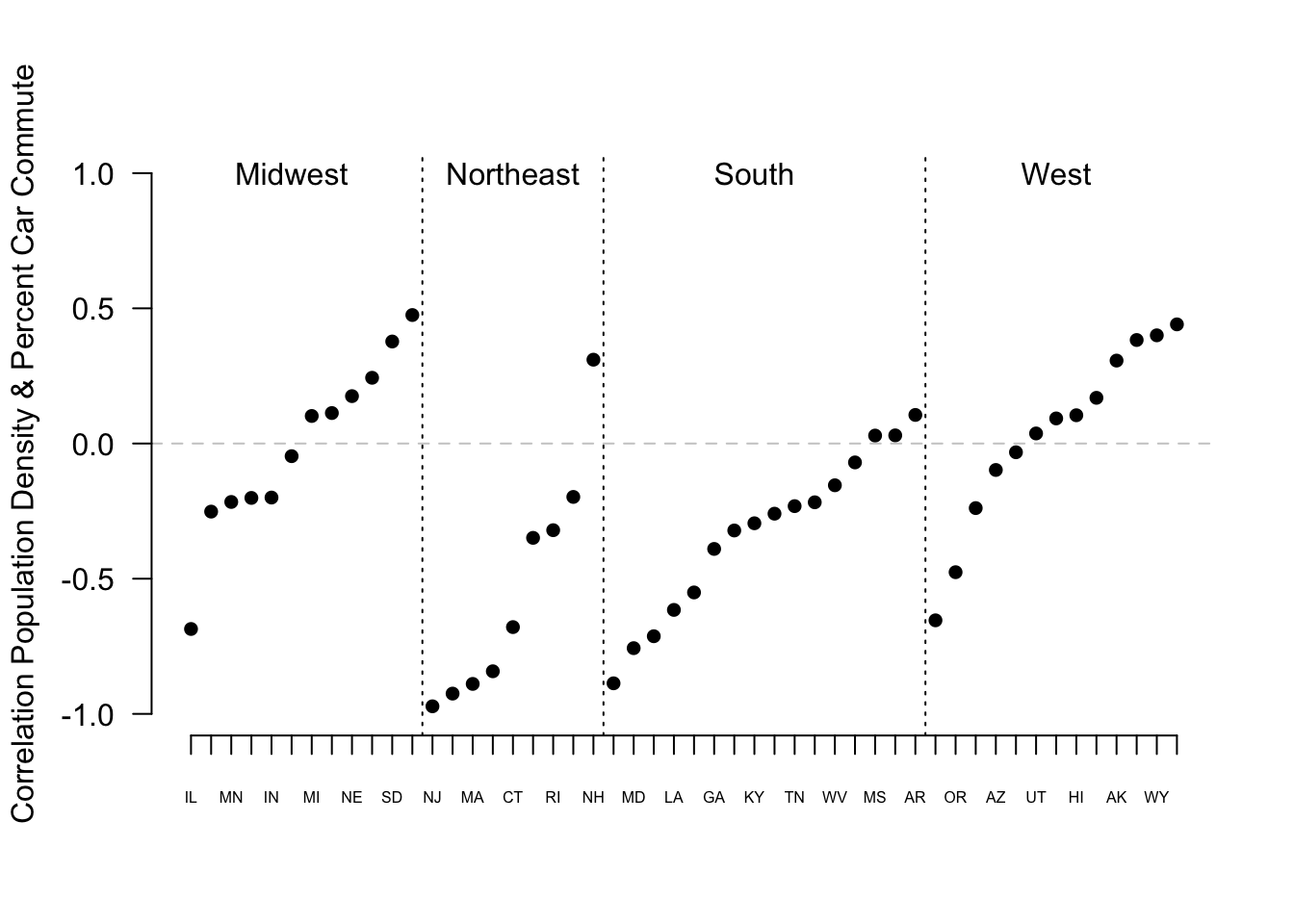
7.2 Double Loops
Things can get really crazy: we can also embed a loop in a loop! This can get complex, but the most important thing to remember is the processes I have taught you. Always try to set things up to perform what you want for the first case without a loop, and then put that in a loop. Remember that you can always take things out of a loop, put in integers, and determine exactly what is going to happen.
What’s the probability of all heads when we flip 2 coins, 3 coins, 4 coins, all they way up to 15 coins. We know that getting all heads is more rare as we flip more coins, but how quickly does the probability drop off?
First: let’s write code to simulate 1000 flips of 2 coins, recording how frequently both come up heads:
Here is how I would do this for the first case:
coin <- c(0,1)
all.heads <- rep(NA, 1000)

flips <- sample(coin, 2, replace=T)
all.heads[1] <- sum(flips)==2
Now let’s put this in a loop:
coin <- c(0,1)

all.heads <- rep(NA, 1000)

for(i in 1:1000){
  flips <- sample(coin, 2, replace=T)
  all.heads[i] <- sum(flips)==2
}
mean(all.heads)
#> [1] 0.243
22% of the time in our simulation we get two heads in two flips. (The truth is that it’s 25% , but simulation is an approximation!)
What would we need to do to change this code to perform the same thing but for 3 heads?
all.heads <- rep(NA, 1000)

for(i in 1:1000){
  flips <- sample(coin, 3, replace=T)
  all.heads[i] <- sum(flips)==3
}
mean(all.heads)
#> [1] 0.132
14% of the time we get all heads with 3 coins
And for 4…
all.heads <- rep(NA, 1000)

for(i in 1:1000){
  flips <- sample(coin, 4, replace=T)
  all.heads[i] <- sum(flips)==4
}
mean(all.heads)
#> [1] 0.064
5.6% of the time we get all heads with 4 coins.
We’re faced, now, with a pretty similar problem as the one that originally caused us to want to make a loop. We need to repeat the same code a bunch of times, each time changing one thing. We could just copy and paste this code 15 times each time changing the number of flips, but that’s super inefficient.
What will do is embed this whole thing in an outer loop to change the number of coins from 2 to 15.
We can’t use i a second time, because that’s already the variable that changes in the inner loop. Convention says to use j as the second looping variable.
num.coins <- seq(2,15,1)
p.all.heads <- rep(NA, length(num.coins))


for(j in 1:length(num.coins)){
  all.heads <- rep(NA, 1000)

  for(i in 1:1000){
    flips <- sample(coin, num.coins[j], replace=T)
    all.heads[i] <- sum(flips)==num.coins[j]
  }
  p.all.heads[j] <-mean(all.heads)
}

plot(num.coins, p.all.heads, type="b")
What’s literally happening inside these loops
Enter the world where j=1:
all.heads <- rep(NA, 1000)

#i counts from 1-1000
flips <- sample(coin, num.coins[1], replace=T)
all.heads[1] <- sum(flips)==num.coins[1]
flips <- sample(coin, num.coins[1], replace=T)
all.heads[2] <- sum(flips)==num.coins[1]
flips <- sample(coin, num.coins[1], replace=T)
all.heads[3] <- sum(flips)==num.coins[1]
flips <- sample(coin, num.coins[1], replace=T)
all.heads[4] <- sum(flips)==num.coins[1]
flips <- sample(coin, num.coins[1], replace=T)
all.heads[5] <- sum(flips)==num.coins[1]
#
#
#
flips <- sample(coin, num.coins[1], replace=T)
all.heads[1000] <- sum(flips)==num.coins[1]

#Save result
p.all.heads[1] <-mean(all.heads)
Enter the world where j=2:
all.heads <- rep(NA, 1000)

#i counts from 1-1000
flips <- sample(coin, num.coins[2], replace=T)
all.heads[1] <- sum(flips)==num.coins[2]
flips <- sample(coin, num.coins[2], replace=T)
all.heads[2] <- sum(flips)==num.coins[2]
flips <- sample(coin, num.coins[2], replace=T)
all.heads[3] <- sum(flips)==num.coins[2]
flips <- sample(coin, num.coins[2], replace=T)
all.heads[4] <- sum(flips)==num.coins[2]
flips <- sample(coin, num.coins[2], replace=T)
all.heads[5] <- sum(flips)==num.coins[2]
#
#
#
flips <- sample(coin, num.coins[2], replace=T)
all.heads[1000] <- sum(flips)==num.coins[2]

#Save result
p.all.heads[2] <-mean(all.heads)
Then it would continue for 3, 4, 5,….,15.
7.3 Extra Loop Examples
Here is a second double loop example:
What if we wanted to create a new ACS dataset that took the mean of all these variables for all of the states. So this same dataset, at the state rather than county level.
I’m going to load a fresh copy of ACS because i’ve created a bunch of stuff above:
acs <- rio::import("https://github.com/marctrussler/IDS-Data/raw/main/ACSCountyData.csv")
names(acs)
#>  [1] "V1"                      "county.fips"
#>  [3] "county.name"             "state.full"
#>  [5] "state.abbr"              "state.alpha"
#>  [7] "state.icpsr"             "census.region"
#>  [9] "population"              "population.density"
#> [11] "percent.senior"          "percent.white"
#> [13] "percent.black"           "percent.asian"
#> [15] "percent.amerindian"      "percent.less.hs"
#> [17] "percent.college"         "unemployment.rate"
#> [19] "median.income"           "gini"
#> [21] "median.rent"             "percent.child.poverty"
#> [23] "percent.adult.poverty"   "percent.car.commute"
#> [25] "percent.transit.commute" "percent.bicycle.commute"
#> [27] "percent.walk.commute"    "average.commute.time"
#> [29] "percent.no.insurance"
What we wantto do is to take averages for all of the variables from population to percent no insurance
We’d want to run code that looks like this, where we want to change both the state and the variable:
mean(acs[acs$state.abbr=="AL", "population"])
#> [1] 72607.16
Let’s create a list of the variables we want means for
vars <- names(acs)[9:28]
vars
#>  [1] "population"              "population.density"
#>  [3] "percent.senior"          "percent.white"
#>  [5] "percent.black"           "percent.asian"
#>  [7] "percent.amerindian"      "percent.less.hs"
#>  [9] "percent.college"         "unemployment.rate"
#> [11] "median.income"           "gini"
#> [13] "median.rent"             "percent.child.poverty"
#> [15] "percent.adult.poverty"   "percent.car.commute"
#> [17] "percent.transit.commute" "percent.bicycle.commute"
#> [19] "percent.walk.commute"    "average.commute.time"
And we know how to make a list of states:
states <- unique(acs$state.abbr)
states
#>  [1] "AL" "AK" "AZ" "AR" "CA" "CO" "CT" "DE" "DC" "FL" "GA"
#> [12] "HI" "ID" "IL" "IN" "IA" "KS" "KY" "LA" "ME" "MD" "MA"
#> [23] "MI" "MN" "MS" "MO" "MT" "NE" "NV" "NH" "NJ" "NM" "NY"
#> [34] "NC" "ND" "OH" "OK" "OR" "PA" "RI" "SC" "SD" "TN" "TX"
#> [45] "UT" "VT" "VA" "WA" "WV" "WI" "WY"
How can we take advantage of the loop functionality to index both of these things?
Let’s try this way first (THIS IS WRONG)
i<- 1
mean(acs[acs$state.abbr==states[i], vars[i]])
#> [1] 72607.16
What would happen if we ran this code in a loop?
That doesn’t work! We are telling R to get the mean of the first state for the first variable, then the mean of the second state for the second variable, mean of the third state for the third variable…
mean(acs[acs$state.abbr==states[1], vars[1]])
#> [1] 72607.16
mean(acs[acs$state.abbr==states[2], vars[2]])
#> [1] 7.880517
Instead we need to say: Ok, R. Start with the first variable (population). For this variable, loop through all of the states. Once you’re finished with that, move on to the second variable and loop through all of the states again.
We want to do something like this, where we are preserving the loop that already works, and thenprogressively working through each variable:
for(i in 1:length(states)){
  mean(acs[acs$state.abbr==states[i], "population"], na.rm=T)
}


for(i in 1:length(states)){
  mean(acs[acs$state.abbr==states[i], "population.density"], na.rm=T)
}


for(i in 1:length(states)){
  mean(acs[acs$state.abbr==states[i], "percent.senior"], na.rm=T)
}
To do so, we want to set up an “outer” loop that moves through the variables
We get something like this:
for(j in 1: length(vars)){
  for(i in 1:length(states)){
    mean(acs[acs$state.abbr==states[i], vars[j]], na.rm=T)
  }
}
Notice that we are now indexing by two objects: i & j. i is indexing states, j is indexing variable names.
So R will start the outside loop with j=1, it will then start the inside loop with i=1, and keep running that inside loop until i=51. Then it will go back to the start of the outside loop and make j=2…
But where are we going to save these estimates? We now have to save them in a matrix with both rows and columns.
Think about what we want to do here: we want to
for(i in 1:length(states)){
  state.demos[i,1] <-  mean(acs[acs$state.abbr==states[i], vars[1]], na.rm=T)
}


for(i in 1:length(states)){
  state.demos[i,2] <-  mean(acs[acs$state.abbr==states[i], vars[2]], na.rm=T)
}


for(i in 1:length(states)){
  state.demos[i,3] <-  mean(acs[acs$state.abbr==states[i], vars[3]], na.rm=T)
}
Notice how the numbers are increasing the same way on the left and right side of the assignment operator
We need to tell R where to save each mean, with the correct row and column:
for(j in 1: length(vars)){

  for(i in 1:length(states)){
    state.demos[i,j] <-  mean(acs[acs$state.abbr==states[i], vars[j]], na.rm=T)
  }

}
It’s easy, then, to combine this matrix with the state names we have saved, and to use the vars vector to create labels.
state.demos <- cbind.data.frame(states,state.demos)

names(state.demos)[2:21] <- vars
Note, additionally, that we could have organized that loop in the opposite way, making the outer loop index through states, and the inner loop index through variables:
This gives the exact same result:
state.demos2 <- matrix(NA, nrow=length(states), ncol=length(vars))


for(i in 1: length(states)){

  for(j in 1:length(vars)){
    state.demos2[i,j] <-  mean(acs[acs$state.abbr==states[i], vars[j]], na.rm=T)
  }

}

state.demos2 <- cbind.data.frame(states,state.demos2)

names(state.demos2)[2:21] <- vars
WARNING: THIS ISN’T ACTUALLY HOW YOU WOULD FIND OUT THE AVERAGE FOR EACH STATE. Just looking at the mean of county values for each of these variables assumes each county is of the same population. They obviously are not!
7.4 If statements
The conditional statements we’ve worked with so far have evaluated our data to say, if this condition holds in this row, take this action. Sometimes we want to extend this and say, if a certain condition holds, Run this code
We can do this via if statements. Similar to when we do this for a single line of code, we start with a logical statment – a statement that produces a single T or F, and then R will only run the code if the statement is True.
So for example:
operation <- "add"
if (operation == "add") {
  print("I'm going to add:")
  4+4
}
#> [1] "I'm going to add:"
#> [1] 8
But if we do the following it won’t work:
operation <- "multiply"

if (operation == "add") {
  print("I'm going to add:")
  4+4

}
Nothing happened here, and that is by design. R thought: in order for me to run this code chunk,this logical statement has to be True, it’s not, so I’ll skip it.
But if we set up a second if statement it will work:
if (operation == "multiply") {
  print("I'm going to multiply:")
  4*4
}
#> [1] "I'm going to multiply:"
#> [1] 16
We can even run both at the same time and only get the one that evaluates as True.
operation <- "multiply"
if (operation == "add") {
  print("I'm going to add:")
  4+4

}
if (operation == "multiply") {
  print("I'm going to multiply:")
  4*4

}
#> [1] "I'm going to multiply:"
#> [1] 16

operation <- "add"

if (operation == "add") {
  print("I'm going to add:")
  4+4

}
#> [1] "I'm going to add:"
#> [1] 8
if (operation == "multiply") {
  print("I'm going to multiply:")
  4*4
}
Right now our if statement says: if condition is True, run code, if it’s not, do nothing. But often times we want to say: if condition is True, run code, if it’s not, run this other code.We can accomplish this by adding an “else”
if(2+2==4){
  print("code chunk 1")
} else {
  print("code chunk 2")
}
#> [1] "code chunk 1"

if(2+2==5){
  print("code chunk 1")
} else {
  print("code chunk 2")
}
#> [1] "code chunk 2"
So if we wanted a chunk of code that adds if we tell it to, but otherwise multiplies:
operation <- "add"

if (operation == "add") {
  print("I'm going to add:")
  4+4

} else {
  print("I'm going to multiply:")
  4*4
}
#> [1] "I'm going to add:"
#> [1] 8

operation <- "subtract"

if (operation == "add") {
  print("I'm going to add:")
  4+4

} else {
  print("I'm going to multiply:")
  4*4
}
#> [1] "I'm going to multiply:"
#> [1] 16
The nice thing about these is they are infinitely stackable using else if ()
operation  <- "subtract"

if (operation == "add") {
  print("I'm going to add:")
  4+4

} else if (operation=="multiply") {
  print("I'm going to multiply:")
  4*4
} else {
  print("Please enter a valid operator.")
}
#> [1] "Please enter a valid operator."
Where is this sort of thing helpful? This is a bit of a “you’ll know it when you see it” situation. Where I use them most is inside loops. For example in election work I am often loading in many snapshots of data from across an election night, and I might only run certain functions when a state has reached a certain threshold of completeness.
Here is an example of where it might be helpful. Here are the 2020 presidential election results by county:
pres <- rio::import("https://github.com/marctrussler/IDS-Data/raw/main/CountyPresData2020.Rds")
#> Warning: Missing `trust` will be set to FALSE by default
#> for RDS in 2.0.0.
What if I want to record the winning margin in each state. That is: regardless of whether Trump or Biden carried the state, how much did they win by?
First, let’s write code that finds the dem and rep margin in each state:
head(pres)
#>   state county fips.code biden.votes trump.votes
#> 1    AK   ED 1     02901        3477        3511
#> 2    AK  ED 10     02910        2727        8081
#> 3    AK  ED 11     02911        3130        7096
#> 4    AK  ED 12     02912        2957        7893
#> 5    AK  ED 13     02913        2666        4652
#> 6    AK  ED 14     02914        4261        6714
#>   other.votes
#> 1         326
#> 2         397
#> 3         402
#> 4         388
#> 5         395
#> 6         468
pres$total.votes <- pres$biden.votes + pres$trump.votes + pres$other.votes

state <- unique(pres$state)
dem.perc <- NA
rep.perc <- NA

i <- 1
for(i in 1:length(state)){
  dem.perc[i] <- sum(pres$biden.votes[pres$state==state[i]])/ sum(pres$total.votes[pres$state==state[i]])
  rep.perc[i] <- sum(pres$trump.votes[pres$state==state[i]])/ sum(pres$total.votes[pres$state==state[i]])

}
results <- cbind.data.frame(state, dem.perc, rep.perc)
Pretty good! But to also calculate the winning margin in each state our code will need to be different dependent on the code of those two columns. Specifically, if the dem is the winner then the winning margin is dem-rep but if the rep is the winner then the winning margin is rep-dem. We can accomplish this via an if statement:
state <- unique(pres$state)
dem.perc <- NA
rep.perc <- NA
winner.margin <- NA
i <- 1
for(i in 1:length(state)){
  dem.perc[i] <- sum(pres$biden.votes[pres$state==state[i]])/ sum(pres$total.votes[pres$state==state[i]])
  rep.perc[i] <- sum(pres$trump.votes[pres$state==state[i]])/ sum(pres$total.votes[pres$state==state[i]])

  if(dem.perc[i]>rep.perc[i]){
    winner.margin[i] <- dem.perc[i]- rep.perc[i]
  } else {
    winner.margin[i] <- rep.perc[i]-dem.perc[i]
  }

}
results <- cbind.data.frame(state,dem.perc, rep.perc, winner.margin)
results <- results[order(results$winner.margin),]
Why would this have been wrong?
state <- unique(pres$state)
dem.perc <- NA
rep.perc <- NA
winner.margin <- NA
i <- 1
for(i in 1:length(state)){
  dem.perc[i] <- sum(pres$biden.votes[pres$state==state[i]])/ sum(pres$total.votes[pres$state==state[i]])
  rep.perc[i] <- sum(pres$trump.votes[pres$state==state[i]])/ sum(pres$total.votes[pres$state==state[i]])

  if(dem.perc[i]>rep.perc[i]){
    winner.margin[i] <- dem.perc[i]- rep.perc[i]
  }
    winner.margin[i] <- rep.perc[i]-dem.perc[i]

}
results <- cbind.data.frame(state,dem.perc, rep.perc, winner.margin)
results <- results[order(results$winner.margin),]
7.5 Minimum Double Loop Example
Here is some election data for multiple years:
x <- rio::import("https://github.com/marctrussler/IDS-Data/raw/main/MITElectionDataPres0016.Rds")
#> Warning: Missing `trust` will be set to FALSE by default
#> for RDS in 2.0.0.
head(x)
#>   year   state state_po  county FIPS    office
#> 1 2000 Alabama       AL Autauga 1001 President
#> 2 2000 Alabama       AL Autauga 1001 President
#> 3 2000 Alabama       AL Autauga 1001 President
#> 4 2000 Alabama       AL Autauga 1001 President
#> 5 2000 Alabama       AL Baldwin 1003 President
#> 6 2000 Alabama       AL Baldwin 1003 President
#>        candidate      party candidatevotes totalvotes
#> 1        Al Gore   democrat           4942      17208
#> 2 George W. Bush republican          11993      17208
#> 3    Ralph Nader      green            160      17208
#> 4          Other         NA            113      17208
#> 5        Al Gore   democrat          13997      56480
#> 6 George W. Bush republican          40872      56480
#>    version
#> 1 20191203
#> 2 20191203
#> 3 20191203
#> 4 20191203
#> 5 20191203
#> 6 20191203
Do a little re-shaping to get to county-year unit of analysis:
x$candidate <- NULL
elect <- pivot_wider(x,
                names_from="party",
                values_from="candidatevotes")
keep <- c("year","state","county","FIPS","democrat","totalvotes")
elect <- elect[keep]
elect.all <- elect
head(elect.all)
#> # A tibble: 6 × 6
#>    year state    county    FIPS democrat totalvotes
#>   <int> <I<chr>> <I<chr>> <int>    <int>      <int>
#> 1  2000 Alabama  Autauga   1001     4942      17208
#> 2  2000 Alabama  Baldwin   1003    13997      56480
#> 3  2000 Alabama  Barbour   1005     5188      10395
#> 4  2000 Alabama  Bibb      1007     2710       7101
#> 5  2000 Alabama  Blount    1009     4977      17973
#> 6  2000 Alabama  Bullock   1011     3395       4904
What is the democratic percent of the vote in every state in every year?
As always, start by doing this for one case. What is the democratic percent of the vote in Alabama in 2000?
sum(elect.all$democrat[elect.all$state=="Alabama" & elect.all$year==2000])/sum(elect.all$totalvotes[elect.all$state=="Alabama" & elect.all$year==2000])
#> [1] 0.4158928
Build from there: how could we calculate the democratic vote in every state in 2000? This is the same sort of loop question that we’ve already been working on:
states <- unique(elect.all$state)

for(i in 1:length(states)){
  sum(elect.all$democrat[elect.all$state==states[i] & elect.all$year==2000])/sum(elect.all$totalvotes[elect.all$state==states[i] & elect.all$year==2000])
}
I’m not going to save this to anything right now, but we can look at it and see that it’s doing what we want.
Now we want to run this code changing the years from 2000 to 2004 etc. Remember, treat the whole block above as the chunk of code we are repeating. We don’t even care that it contains a loop:
years <- unique(elect.all$year)
states <- unique(elect.all$state)

for(j in 1:length(years)){
  for(i in 1:length(states)){
    sum(elect.all$democrat[elect.all$state==states[i] & elect.all$year==years[j]])/sum(elect.all$totalvotes[elect.all$state==states[i] & elect.all$year==years[j]])
  }
}
Finally we have to save what we’ve done here. Because we want a data entry point for each state in each year, we have to create a matrix. I’m going to create an empty matrix that has a row for each state and a column for each year. Then I have to save each percent in the right slot. This is the hardest part! But go slowly and draw it on a piece of paper if you have to.
years <- unique(elect.all$year)
states <- unique(elect.all$state)
result <- matrix(NA, nrow = length(states), ncol=length(years))

for(j in 1:length(years)){
  for(i in 1:length(states)){
    result[i,j] <- sum(elect.all$democrat[elect.all$state==states[i] & elect.all$year==years[j]],na.rm=T)/sum(elect.all$totalvotes[elect.all$state==states[i] & elect.all$year==years[j]],na.rm=T)
  }
}
result
#>            [,1]      [,2]      [,3]      [,4]      [,5]
#>  [1,] 0.4158928 0.3684440 0.3874043 0.3843287 0.3435803
#>  [2,] 0.4467344 0.4439683 0.4511525 0.4458977 0.4417173
#>  [3,] 0.4586426 0.4447506 0.3886466 0.3687899 0.3367513
#>  [4,] 0.5344957 0.5440512 0.6101264 0.6023896 0.6172640
#>  [5,] 0.4239358 0.4703784 0.5366024 0.5149421 0.4815698
#>  [6,] 0.5590963 0.5431371 0.6073099 0.5791526 0.5439909
#>  [7,] 0.5497773 0.5334675 0.6194267 0.5860409 0.5318388
#>  [8,] 0.8515508 0.8918387 0.9245711 0.9091311 0.9086382
#>  [9,] 0.4884387 0.4709111 0.5103134 0.5000787 0.4782332
#> [10,] 0.4298476 0.4141364 0.4698105 0.4548216 0.4564022
#> [11,] 0.5579184 0.5398024 0.7182921 0.7053229 0.6222149
#> [12,] 0.2763780 0.3026492 0.3609595 0.3262233 0.2748493
#> [13,] 0.5459635 0.5482012 0.6191638 0.5760349 0.5560158
#> [14,] 0.4101205 0.3926297 0.4994591 0.4392730 0.3777484
#> [15,] 0.4853565 0.4923313 0.5393865 0.5198802 0.4174049
#> [16,] 0.3723839 0.3662309 0.4165197 0.3804597 0.3605234
#> [17,] 0.4137439 0.3968756 0.4117064 0.3780133 0.3268219
#> [18,] 0.4487533 0.4221586 0.3989485 0.4057746 0.3844957
#> [19,] 0.4908602 0.5304409 0.5770574 0.5117583 0.4776187
#> [20,] 0.5656842 0.5591425 0.6191934 0.6197419 0.6032574
#> [21,] 0.5980379 0.6193543 0.6179472 0.6065124 0.6093029
#> [22,] 0.5127725 0.5123071 0.5743130 0.5420820 0.4727453
#> [23,] 0.4790557 0.5109009 0.5406029 0.5265230 0.4644492
#> [24,] 0.4070293 0.3946992 0.4315566 0.4378936 0.4011479
#> [25,] 0.4708427 0.4610045 0.4929265 0.4438366 0.3815186
#> [26,] 0.3336513 0.3856503 0.4679885 0.4170813 0.3574577
#> [27,] 0.3325304 0.3268216 0.4159827 0.3802731 0.3370035
#> [28,] 0.4597566 0.4787804 0.5514668 0.5235625 0.4791782
#> [29,] 0.4680318 0.5024791 0.5412690 0.5198268 0.4682626
#> [30,] 0.5612561 0.5295273 0.5771586 0.5837721 0.5545308
#> [31,] 0.4790855 0.4904668 0.5690748 0.5299276 0.4825565
#> [32,] 0.6021251 0.5656521 0.6283169 0.6123299 0.5900283
#> [33,] 0.4320092 0.4358315 0.4970438 0.4835097 0.4617287
#> [34,] 0.3305408 0.3549881 0.4462054 0.3869731 0.2722674
#> [35,] 0.4646074 0.4870479 0.5148058 0.5066675 0.4355808
#> [36,] 0.3842690 0.3442960 0.3435492 0.3322768 0.2893168
#> [37,] 0.4695939 0.5134866 0.5674881 0.5423933 0.5007185
#> [38,] 0.5060817 0.5095760 0.5464258 0.5207686 0.4785362
#> [39,] 0.6098770 0.5953852 0.6286400 0.5375690 0.5390397
#> [40,] 0.4090536 0.4090293 0.4489656 0.4408803 0.4067342
#> [41,] 0.3756423 0.3844365 0.4525295 0.3986614 0.3173743
#> [42,] 0.4728489 0.4249794 0.4182251 0.3907581 0.3471633
#> [43,] 0.3798196 0.3822426 0.4368312 0.4138336 0.4323526
#> [44,] 0.2634472 0.2599564 0.3440575 0.2474967 0.2745870
#> [45,] 0.5063471 0.5893746 0.6745568 0.6657055 0.5667599
#> [46,] 0.4442877 0.4548390 0.5262947 0.5115646 0.4972789
#> [47,] 0.5013790 0.5282115 0.5765289 0.5616340 0.5430358
#> [48,] 0.4559266 0.4321275 0.4258975 0.3553920 0.2647693
#> [49,] 0.4783282 0.4969972 0.5621779 0.5277616 0.4643608
#> [50,] 0.2769898 0.2907472 0.3236589 0.2781889 0.2187736
#> [51,] 0.2766925 0.3690763 0.3788937 0.3274417 0.3604137