8 Review
The best way to review for the midterm will be to read the notes in this book and to carefully go through the problem set questions. As I mentioned in class, it’s also helpful to literally write out the code that is in the textbook, to help build repetitions in coding and eliminate the sort of small errors that can derail you in a timed midterm.
All of the questions in the problem sets are designed to be straight-forward applications of the class material. Oftentimes they are just class examples with re-named variables. Try to think about what different parts of the examples are doing. Try to edit things and see if they still work. For ex. an example makes deciles of population density, what if I made deciles of income instead?
The midterm questions will similarly be straight-forward applications of class examples. There may be cases where things are presented in a new form or combine concepts, but if you have a grasp of the in-class and problem set code there will be absolutely nothing surprising about the midterm.
My other tips for the midterm are: knit your rmarkdown often so you don’t get stuck at the end; read every question fully before starting; pay attention to extra information I’ve provided; pay attention to the words I use in the questions and how those words relate to the course material; make sure to put something down for absolutely every question (I can’t give partial credit if you have literally 0 things written).
8.1 Broad view of the course
Here are some brief notes and examples to give a very broad view of what I hope for you to pick up in each chapter. This is designed to give you a sense of what I think each chapter is about and what I want you to learn. The following is definitely not sufficient for studying.
8.1.1 What is Data?
The focus of this chapter was to have you think through what the ultimate goals of data science and statistics are. In this class we are going to spend a lot of time manipulating individual datasets which is not the purpose of statistics. The purpose of statistics is to use the sample of data that we have to make inferences about broader populations. The way these inferences work is by understanding that our dataset is one of an infinite number of datasets that could exist, and therefore everything that we calculate has some degree of sampling variability. We want to make inferences about the likelihood of observing our data given assumptions about the truth and a measure of sampling variability.
8.1.2 Basic R
A broad understanding of why we are using R, and why the use of scripts is key for replicability.
Using R as a basic calculator.
4 + 2
#> [1] 6
2 + sqrt(4)
#> [1] 4- Creating objects, including individual numbers, vectors, and matrices.
- The use of functions to operate on those objects
mean(x)
#> [1] 3- The use of square brackets to access information stored in objects.
y[3]
#> [1] 3
dat[1,2]
#> z
#> 4
dat[1,]
#> y z
#> 1 4
dat[,1]
#> [1] 1 2 3- Basic plots including barplots, boxplots, and scatterplots.
plot(dat[,1], dat[,2])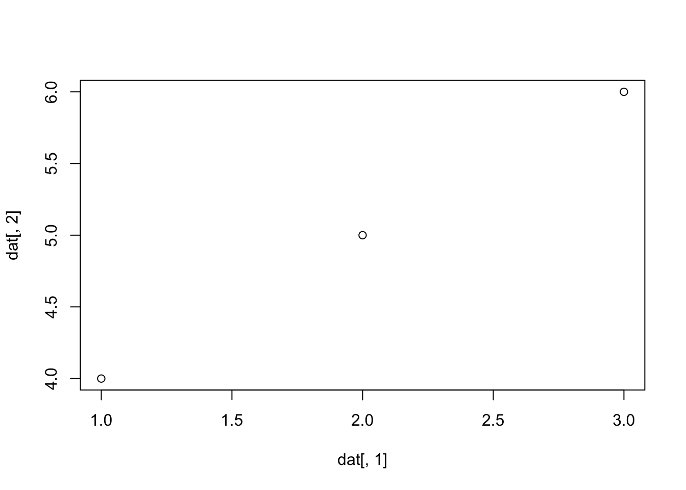
8.1.3 Conditional Logic
- Using logical statements to create boolean variables (
==, >,<, !, %in%)
3>4
#> [1] FALSE
3==sqrt(9)
#> [1] TRUE- Using boolean variables to subset existing data.
dat[dat[,1]>1,]
#>      y z
#> [1,] 2 5
#> [2,] 3 6- Stringing together multiple logical statemetns with
&, |.
3==3 & 3==4
#> [1] FALSE
3==3 | 3==4
#> [1] TRUE- Boolean variables are treated as 1s and 0s, which means that we can use them to determine probability of events:
x <- 1:10
x<5
#>  [1]  TRUE  TRUE  TRUE  TRUE FALSE FALSE FALSE FALSE FALSE
#> [10] FALSE
sum(x<5)
#> [1] 4
mean(x<5)
#> [1] 0.4- Making plots with conditional logic.
8.1.4 Data Frames
acs <- rio::import("https://github.com/marctrussler/IDS-Data/raw/main/ACSCountyData.csv", trust=T)Understanding the use case for a data frame over a “sample” matrix created with
cbind()The use of named columns to access variables in a dataset.
head(acs$population)
#> [1] 102939 23875 37328 55200 208107 25782- Extending our knowledge of square brackets and conditional logic to data frames.
acs$population[acs$population>1E7]
#> [1] 10098052- The use of
which()to determine rows that match a condition.
which(acs$percent.transit.commute>40)
#> [1] 1785 1834 1855 1862 1872- Using conditional logic to recode variables.
acs$high.transit <- NA
acs$high.transit[acs$percent.transit.commute>30] <- 1
#Or
acs$high.transit <- acs$percent.transit.commute>30
Understanding and preserving missing data.
Converting dates to the right class.
lubridate::ymd("2020-02-01")
#> [1] "2020-02-01"- Editing and cleaning character information.
gsub("_","","test_test")
#> [1] "testtest"
tolower("BBB")
#> [1] "bbb"
toupper("ccc")
#> [1] "CCC"

out <- separate(acs,
                "county.name",
                into = c("county","extra"),
                sep=" ")
#> Warning in gregexpr(pattern, x, perl = TRUE): input string
#> 1805 is invalid UTF-8
#> Warning: Expected 2 pieces. Additional pieces discarded in 209 rows
#> [57, 68, 69, 70, 71, 73, 74, 76, 77, 79, 80, 81, 82, 83,
#> 84, 85, 87, 88, 89, 91, ...].
#> Warning: Expected 2 pieces. Missing pieces filled with `NA` in 1
#> rows [1805].
head(out$county)
#> [1] "Etowah"   "Winston"  "Escambia" "Autauga"  "Baldwin"
#> [6] "Barbour"
8.1.5 Cleaning and Reshaping
- Reshaping data using the
pivotcommands.
dat <- rio::import("https://github.com/marctrussler/IDS-Data/raw/main/WideExample.RDS")
#> Warning: Missing `trust` will be set to FALSE by default
#> for RDS in 2.0.0.
dat
#>   county date_1_1_2021 date_1_2_2021 date_1_3_2021
#> 1     c1           990             9           215
#> 2     c2           140          1000           305
#> 3     c3           797           323           141
#> 4     c4           343            34           645
#>   date_1_4_2021
#> 1           646
#> 2             4
#> 3           260
#> 4           785
#Wide to Long
dat.l <- pivot_longer(dat,cols=date_1_1_2021:date_1_4_2021,
                      names_to = "date",
                      values_to = "covid.cases")
dat.l
#> # A tibble: 16 × 3
#>    county date          covid.cases
#>    <chr>  <chr>               <dbl>
#>  1 c1     date_1_1_2021         990
#>  2 c1     date_1_2_2021           9
#>  3 c1     date_1_3_2021         215
#>  4 c1     date_1_4_2021         646
#>  5 c2     date_1_1_2021         140
#>  6 c2     date_1_2_2021        1000
#>  7 c2     date_1_3_2021         305
#>  8 c2     date_1_4_2021           4
#>  9 c3     date_1_1_2021         797
#> 10 c3     date_1_2_2021         323
#> 11 c3     date_1_3_2021         141
#> 12 c3     date_1_4_2021         260
#> 13 c4     date_1_1_2021         343
#> 14 c4     date_1_2_2021          34
#> 15 c4     date_1_3_2021         645
#> 16 c4     date_1_4_2021         785
#Long to Wide 1
pivot_wider(dat.l,
             names_from="county",
             values_from="covid.cases")
#> # A tibble: 4 × 5
#>   date             c1    c2    c3    c4
#>   <chr>         <dbl> <dbl> <dbl> <dbl>
#> 1 date_1_1_2021   990   140   797   343
#> 2 date_1_2_2021     9  1000   323    34
#> 3 date_1_3_2021   215   305   141   645
#> 4 date_1_4_2021   646     4   260   785
#Long to Wide 2
pivot_wider(dat.l,
             names_from="date",
             values_from="covid.cases")
#> # A tibble: 4 × 5
#>   county date_1_1_2021 date_1_2_2021 date_1_3_2021
#>   <chr>          <dbl>         <dbl>         <dbl>
#> 1 c1               990             9           215
#> 2 c2               140          1000           305
#> 3 c3               797           323           141
#> 4 c4               343            34           645
#> # ℹ 1 more variable: date_1_4_2021 <dbl>- Using commands like
duplicatedorncharto find errors/unwanted information in a dataset.
table(duplicated(acs$county.name))
#>
#> FALSE  TRUE
#>  1877  1265
table(nchar(acs$county.fips))
#>
#>    4    5
#>  316 2826
Renaming variable names to properly formatted names.
Basic analysis of data
#Scatterplots
plot(acs$percent.white, acs$median.income,
     main="County Race and Income",
     xlab = "Percent White",
     ylab="Median Income")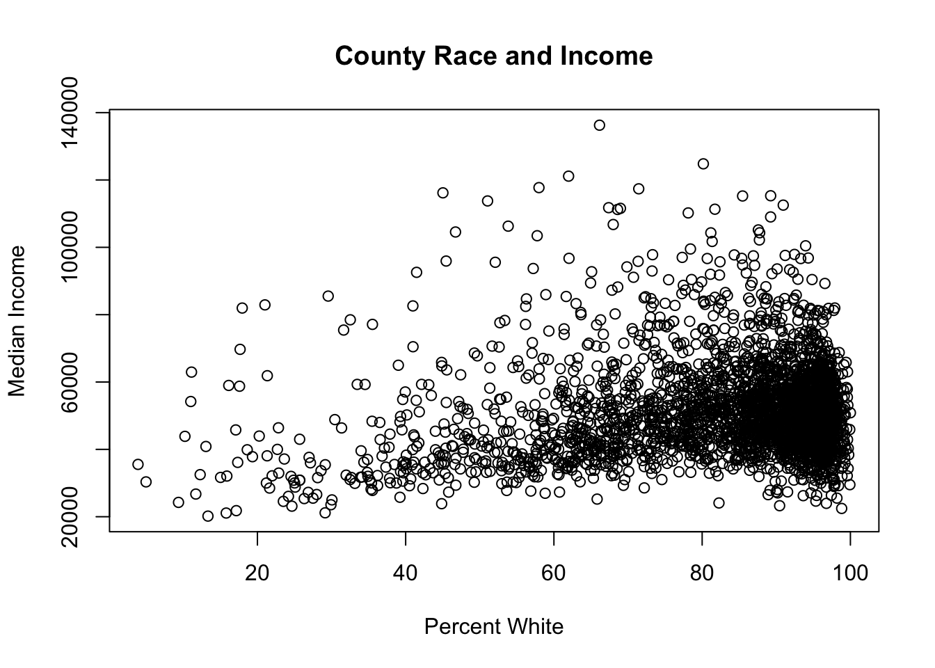
#Boxplots
boxplot(acs$median.income, outline=F)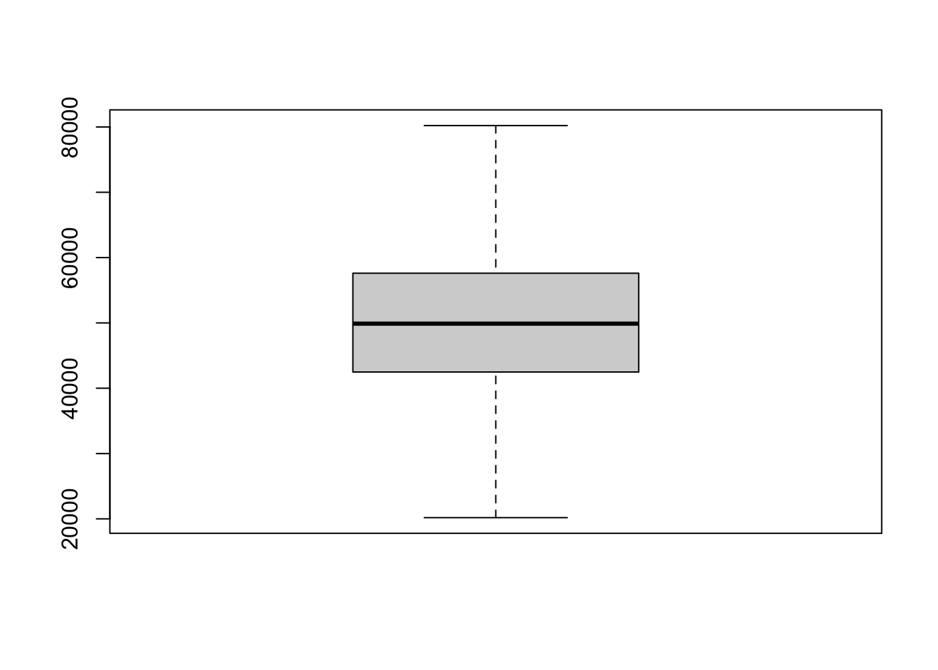
boxplot(acs$median.income ~ acs$census.region, outline=F)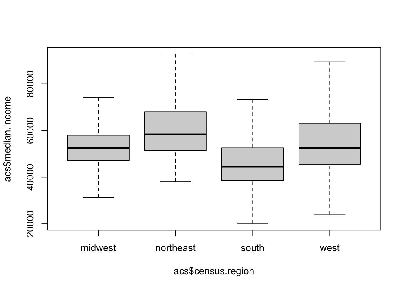
#Density plots
plot(density(acs$median.income[acs$census.region=="south"],na.rm=T), col="firebrick",
     main="Distribution of County Median Income, by Region ")
points(density(acs$median.income[!acs$census.region=="south"],na.rm=T), type="l", col="forestgreen")
legend("topright", c("South","Non-South"), lty=c(1,1), col=c("firebrick","forestgreen"))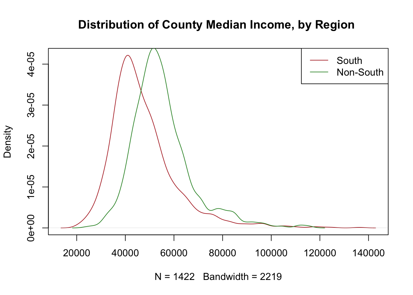
#Correlation
cor(acs$median.income, acs$percent.white,
    use="pairwise.complete")
#> [1] 0.1368011
8.1.6 For Loops
- The use of
for()loops to aggregate data to a higher level.
state <- unique(acs$state.abbr)
avg.poverty <- rep(NA, length(state))
avg.income <- rep(NA, length(state))

for(i in 1:length(state)){
 avg.poverty[i] <- mean(acs$percent.adult.poverty[acs$state.abbr==state[i]], na.rm=T)
 avg.income[i] <- mean(acs$median.income[acs$state.abbr==state[i]], na.rm=T)
}

plot(avg.income, avg.poverty, main="Income Level vs. Poverty Rates",
     ylab="Average Median Income", xlab = "Percent Adults in Poverty",
     type="n")
text(avg.income, avg.poverty, labels = state)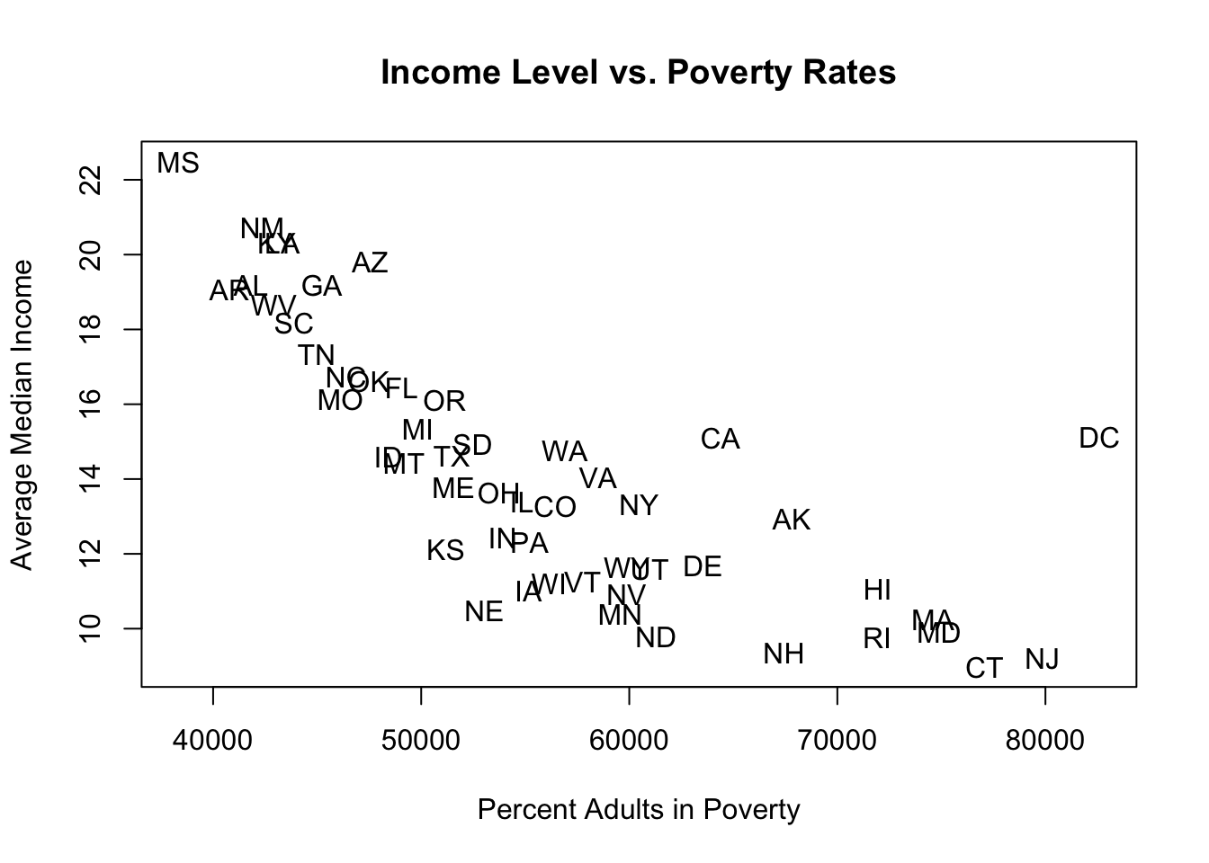
- The use of
for()loops to work on chunks of data in a dataset one at a time.
#What is each counties income level as a percent of it's state average?

acs$rel.income <- NA

for(i in 1:length(state)){
  acs$rel.income[acs$state.abbr==state[i]] <- acs$median.income[acs$state.abbr==state[i]]/mean(acs$median.income[acs$state.abbr==state[i]],na.rm=T)
}

summary(acs$rel.income)
#>    Min. 1st Qu.  Median    Mean 3rd Qu.    Max.    NA's
#> 0.4623 0.8625 0.9660 1.0000 1.0966 2.7209 1- The use of
for()loops to simulate probability.
#What is probability of getting dealt two aces?
#There are 52 cards in the deck and 4 aces
deck <- c(rep("NotAce",48), rep("Ace",4))

#One draw of two cards, check if all equal Ace
draw <- sample(deck, 2, replace=F)
draw=="Ace"
#> [1] FALSE FALSE
all(draw=="Ace")
#> [1] FALSE

#Simulate:
result <- NA
for(i in 1:100000){
draw <- sample(deck, 2, replace=F)
result[i] <- all(draw=="Ace")
}

mean(result)
#> [1] 0.00435

#Half a percent chance