11 Tidyverse I
Updated for S2026? Yes.
#install.packages("tidyverse")
library(tidyverse)
acs <- rio::import("https://github.com/marctrussler/IDS-Data/raw/refs/heads/main/ACSCountyData.csv")
The “tidyverse” is, in the words of it’s own website “an opinionated collection of R packages designed for data science”. It represents a fundamentally different coding philosophy then the one found in base R that we have learned up until this point. The things that we have learned in base R – loading, cleaning, reshaping, combining, and summarizing data – all have a parallel process in tidyverse.
In base R you now have the skills to do the following with the ACS data. Focusing on the southern states, create a new variable which indicates whether more than 10% of a county doesn’t have health insurance, and then find the average of that variable for each state:
acs.south <- acs[acs$census.region=="south",]

acs.south$high.uninsured <- acs.south$percent.no.insurance>10

states <- unique(acs.south$state.abbr)
avg.high.uninsured <- rep(NA, length(states))

for(i in 1:length(states)){
  avg.high.uninsured[i] <- mean(acs.south$high.uninsured[acs.south$state.abbr==states[i]])
}

cbind(states, avg.high.uninsured)
#>       states avg.high.uninsured
#>  [1,] "AL"   "0.537313432835821"
#>  [2,] "AR"   "0.2"
#>  [3,] "DE"   "0"
#>  [4,] "DC"   "0"
#>  [5,] "FL"   "0.82089552238806"
#>  [6,] "GA"   "0.924528301886792"
#>  [7,] "KY"   "0.025"
#>  [8,] "LA"   "0.71875"
#>  [9,] "MD"   "0.0416666666666667"
#> [10,] "MS"   "0.865853658536585"
#> [11,] "NC"   "0.82"
#> [12,] "OK"   "0.935064935064935"
#> [13,] "SC"   "0.717391304347826"
#> [14,] "TN"   "0.4"
#> [15,] "TX"   "0.960629921259842"
#> [16,] "VA"   "0.451127819548872"
#> [17,] "WV"   "0"
To get the equivalent result in tidyverse (you don’t have to know any of this yet, but will at the end of the two weeks!):
acs |>
  filter(census.region=="south") |>
  mutate(high.uninsured=percent.no.insurance>10) |>
  group_by(state.abbr) |>
  summarise(avg.high.uninsured=mean(high.uninsured))
#> # A tibble: 17 × 2
#>    state.abbr avg.high.uninsured
#>    <chr>                   <dbl>
#>  1 AL                     0.537
#>  2 AR                     0.2
#>  3 DC                     0
#>  4 DE                     0
#>  5 FL                     0.821
#>  6 GA                     0.925
#>  7 KY                     0.025
#>  8 LA                     0.719
#>  9 MD                     0.0417
#> 10 MS                     0.866
#> 11 NC                     0.82
#> 12 OK                     0.935
#> 13 SC                     0.717
#> 14 TN                     0.4
#> 15 TX                     0.961
#> 16 VA                     0.451
#> 17 WV                     0
When teaching R I try very hard to not give you two ways of doing things. You are in a steep part of the learning curve, and I have often found it counter-productive to give you two different ways of accomplishing the same thing. Yet, here we go re-learning everything we have done up to this point in a different “grammar”.
Why am I doing this? Why know the tidyverse?
To be clear, there is nothing you can do in the tidyverse that you can’t do in Base R and vice-versa. Rather, I look at the two branches of the language having different advantages and disadvantages.
An advantage to Base R is that it is the language that R actually speaks. We can directly manipulate vectors and matrices quickly and efficiently.
An advantage to Base R is the use of loops, which very clearly and intuitively allow us to repeat the same code many times.
An advantage of Base R is that it is very easy to find coding errors because the code is in discrete chunks.
A disadvantage of Base R is that all of the code exists in discrete, often redundant, chunks that can be messy to read.
A disadvantage of Base R is that the syntax can feel “backwards” or inside out.
acs$high.insurance <- NA
acs$high.insurance[acs$percent.no.insurance<20] <- "Yes"
“Recode the high insurance variable, when percent no insurance is less than 20, to the value”yes”.” Is not how I would tell you to do that process in the english language.
An advantage of tidyverse is that it has very clean prepackaged syntax for basic data manipulation that does the “dirty work” of vector and matrix manipulation for you.
An advantage of tidyverse is that it has very clean syntax for working with groups in your data.
An advantage of tidyverse is that it uses the “pipe” to string together multiple commands to make more efficient code.
A disadvantage of tidyverse is that it can become very frustrating to do anything that deviates from what the designers “expect” you to do.
A disadvantage of tidyverse is that it can be complicated to de-bug code.
A disadvantage of tidyverse is that the “Functional Programming” style has its own steep learning curve.
In previous versions of the class I would just teach base R. But as I increasingly use tidyverse in my own work, it seems wrong to leave it out of the class.
Ultimately: the best R coders seamlessly combine the advantages of the two languages while avoiding the disadvantages. There are dogmatic people on both sides who say that you should stick to one of the two methods fully, which I think is foolish. There are helpful tools in both styles that you can make use of, but you should never feel bad for reaching for the tool that will quickly and efficiently solve the problem you are trying to solve.
11.1 Data transformation
These notes are largely a re-hashing of the excellent resource R for Data Science.
To start working with the tidyverse functions we are going to load in the nycflights13 package, which (unsurprisingly) includes data about flights to and from NYCs airports:
#install.packages("nycflights13")
library(nycflights13)
#Load this data into our environment
data(flights)
The glimpse function is like head, but gives us all the columns.
glimpse(flights)
#> Rows: 336,776
#> Columns: 19
#> $ year           <int> 2013, 2013, 2013, 2013, 2013, 2013,…
#> $ month          <int> 1, 1, 1, 1, 1, 1, 1, 1, 1, 1, 1, 1,…
#> $ day            <int> 1, 1, 1, 1, 1, 1, 1, 1, 1, 1, 1, 1,…
#> $ dep_time       <int> 517, 533, 542, 544, 554, 554, 555, …
#> $ sched_dep_time <int> 515, 529, 540, 545, 600, 558, 600, …
#> $ dep_delay      <dbl> 2, 4, 2, -1, -6, -4, -5, -3, -3, -2…
#> $ arr_time       <int> 830, 850, 923, 1004, 812, 740, 913,…
#> $ sched_arr_time <int> 819, 830, 850, 1022, 837, 728, 854,…
#> $ arr_delay      <dbl> 11, 20, 33, -18, -25, 12, 19, -14, …
#> $ carrier        <chr> "UA", "UA", "AA", "B6", "DL", "UA",…
#> $ flight         <int> 1545, 1714, 1141, 725, 461, 1696, 5…
#> $ tailnum        <chr> "N14228", "N24211", "N619AA", "N804…
#> $ origin         <chr> "EWR", "LGA", "JFK", "JFK", "LGA", …
#> $ dest           <chr> "IAH", "IAH", "MIA", "BQN", "ATL", …
#> $ air_time       <dbl> 227, 227, 160, 183, 116, 150, 158, …
#> $ distance       <dbl> 1400, 1416, 1089, 1576, 762, 719, 1…
#> $ hour           <dbl> 5, 5, 5, 5, 6, 5, 6, 6, 6, 6, 6, 6,…
#> $ minute         <dbl> 15, 29, 40, 45, 0, 58, 0, 0, 0, 0, …
#> $ time_hour      <dttm> 2013-01-01 05:00:00, 2013-01-01 05…
We have already worked with some function from the tidyverse, which all actually come from the package dplyr (a part of the tidyverse). For example seperate and pivot_longer are actually tidyverse functions. We saw with those there were certain similarities, which they will share with other tidyverse commands:
The first argument is always a dataframe.
The subsequent arguments describe which columns to operate on using variable names (without quotes).
The output is always a new data frame.
The reason for this change is it allows for a different form of programming where we can make several changes to a dataframe in one larger step, rather than splitting things into sub-steps like we have been doing. This has the potential to make things clearer in terms of what you are doing (though not always), and has the potential to speed up our coding (though not always).
We can seperate the dplyr/tidyverse “verbs” (what they call functions) into whether they operate on rows, columns, groups, or tables. We will take these on one at a time over the next few classes.
11.1.1 Verbs that operate on rows
The first set of commands we are going to look at are those that operate on rows of data.
For example, what if we want to subset to the rows where dep_delay is greater than 120 minutes?
In traditional R we use a logical statement inside square brackets:
flights[flights$dep_delay>120,]
#> # A tibble: 17,978 × 19
#>     year month   day dep_time sched_dep_time dep_delay
#>    <int> <int> <int>    <int>          <int>     <dbl>
#>  1  2013     1     1      848           1835       853
#>  2  2013     1     1      957            733       144
#>  3  2013     1     1     1114            900       134
#>  4  2013     1     1     1540           1338       122
#>  5  2013     1     1     1815           1325       290
#>  6  2013     1     1     1842           1422       260
#>  7  2013     1     1     1856           1645       131
#>  8  2013     1     1     1934           1725       129
#>  9  2013     1     1     1938           1703       155
#> 10  2013     1     1     1942           1705       157
#> # ℹ 17,968 more rows
#> # ℹ 13 more variables: arr_time <int>,
#> #   sched_arr_time <int>, arr_delay <dbl>, carrier <chr>,
#> #   flight <int>, tailnum <chr>, origin <chr>, dest <chr>,
#> #   air_time <dbl>, distance <dbl>, hour <dbl>,
#> #   minute <dbl>, time_hour <dttm>
In tidyverse we will use the filter() command: For tidyverse remember that our first argument is a dataframe, and the output is also a dataframe. Subsequent arguments describe which columns to operate on, which we can refer to without quotation marks:
filter(flights, dep_delay>120)
#> # A tibble: 9,723 × 19
#>     year month   day dep_time sched_dep_time dep_delay
#>    <int> <int> <int>    <int>          <int>     <dbl>
#>  1  2013     1     1      848           1835       853
#>  2  2013     1     1      957            733       144
#>  3  2013     1     1     1114            900       134
#>  4  2013     1     1     1540           1338       122
#>  5  2013     1     1     1815           1325       290
#>  6  2013     1     1     1842           1422       260
#>  7  2013     1     1     1856           1645       131
#>  8  2013     1     1     1934           1725       129
#>  9  2013     1     1     1938           1703       155
#> 10  2013     1     1     1942           1705       157
#> # ℹ 9,713 more rows
#> # ℹ 13 more variables: arr_time <int>,
#> #   sched_arr_time <int>, arr_delay <dbl>, carrier <chr>,
#> #   flight <int>, tailnum <chr>, origin <chr>, dest <chr>,
#> #   air_time <dbl>, distance <dbl>, hour <dbl>,
#> #   minute <dbl>, time_hour <dttm>
We can read this as: let’s filter the flights data down to when the dep_delay variable in that dataframe is greater than 120. Because dep_delay is a column in flights we don’t need to use the $ operator to refer to it. We’ve already told R the dataframe we are working form is flights. (Indeed, tidyverse doesn’t use $ at all.)
We can, similar to base R, combine logical statements using & and |:
filter(flights, month==1 & day==1)
#> # A tibble: 842 × 19
#>     year month   day dep_time sched_dep_time dep_delay
#>    <int> <int> <int>    <int>          <int>     <dbl>
#>  1  2013     1     1      517            515         2
#>  2  2013     1     1      533            529         4
#>  3  2013     1     1      542            540         2
#>  4  2013     1     1      544            545        -1
#>  5  2013     1     1      554            600        -6
#>  6  2013     1     1      554            558        -4
#>  7  2013     1     1      555            600        -5
#>  8  2013     1     1      557            600        -3
#>  9  2013     1     1      557            600        -3
#> 10  2013     1     1      558            600        -2
#> # ℹ 832 more rows
#> # ℹ 13 more variables: arr_time <int>,
#> #   sched_arr_time <int>, arr_delay <dbl>, carrier <chr>,
#> #   flight <int>, tailnum <chr>, origin <chr>, dest <chr>,
#> #   air_time <dbl>, distance <dbl>, hour <dbl>,
#> #   minute <dbl>, time_hour <dttm>

filter(flights, month==1 | month==2)
#> # A tibble: 51,955 × 19
#>     year month   day dep_time sched_dep_time dep_delay
#>    <int> <int> <int>    <int>          <int>     <dbl>
#>  1  2013     1     1      517            515         2
#>  2  2013     1     1      533            529         4
#>  3  2013     1     1      542            540         2
#>  4  2013     1     1      544            545        -1
#>  5  2013     1     1      554            600        -6
#>  6  2013     1     1      554            558        -4
#>  7  2013     1     1      555            600        -5
#>  8  2013     1     1      557            600        -3
#>  9  2013     1     1      557            600        -3
#> 10  2013     1     1      558            600        -2
#> # ℹ 51,945 more rows
#> # ℹ 13 more variables: arr_time <int>,
#> #   sched_arr_time <int>, arr_delay <dbl>, carrier <chr>,
#> #   flight <int>, tailnum <chr>, origin <chr>, dest <chr>,
#> #   air_time <dbl>, distance <dbl>, hour <dbl>,
#> #   minute <dbl>, time_hour <dttm>
Critically, all that we have done with these commands is to perform the filter and printed the result, we haven’t actually made any changes to the flights dataset. We could write over flights with our new, filtered, dataset. Instead, we are going to save a new dataset that is just the flights on January 1st:
jan1 <- filter(flights, month==1 & day ==1)We can see in our environment that this new dataset is saved and has (appropriately) way fewer rows.
A special type of filter is when we want to subset down to unique rows. We can do that with the distinct() verb. If we just run this on the whole dataset it will remove any rows that are total duplicates. (There aren’t in this dataset):
distinct(flights)
#> # A tibble: 336,776 × 19
#>     year month   day dep_time sched_dep_time dep_delay
#>    <int> <int> <int>    <int>          <int>     <dbl>
#>  1  2013     1     1      517            515         2
#>  2  2013     1     1      533            529         4
#>  3  2013     1     1      542            540         2
#>  4  2013     1     1      544            545        -1
#>  5  2013     1     1      554            600        -6
#>  6  2013     1     1      554            558        -4
#>  7  2013     1     1      555            600        -5
#>  8  2013     1     1      557            600        -3
#>  9  2013     1     1      557            600        -3
#> 10  2013     1     1      558            600        -2
#> # ℹ 336,766 more rows
#> # ℹ 13 more variables: arr_time <int>,
#> #   sched_arr_time <int>, arr_delay <dbl>, carrier <chr>,
#> #   flight <int>, tailnum <chr>, origin <chr>, dest <chr>,
#> #   air_time <dbl>, distance <dbl>, hour <dbl>,
#> #   minute <dbl>, time_hour <dttm>
But if we put variables into this command, if will tell us the distinct (i.e. unique) values for that variable:
distinct(flights, dest)
#> # A tibble: 105 × 1
#>    dest
#>    <chr>
#>  1 IAH
#>  2 MIA
#>  3 BQN
#>  4 ATL
#>  5 ORD
#>  6 FLL
#>  7 IAD
#>  8 MCO
#>  9 PBI
#> 10 TPA
#> # ℹ 95 more rows
We can combine variables to give unique combos of those variables:
distinct(flights, origin, dest)
#> # A tibble: 224 × 2
#>    origin dest
#>    <chr>  <chr>
#>  1 EWR    IAH
#>  2 LGA    IAH
#>  3 JFK    MIA
#>  4 JFK    BQN
#>  5 LGA    ATL
#>  6 EWR    ORD
#>  7 EWR    FLL
#>  8 LGA    IAD
#>  9 JFK    MCO
#> 10 LGA    ORD
#> # ℹ 214 more rows
If we add the option .keep_all=T, it will still print out all of the columns. It will give us the row that is the first occurrence of that unique combination, deleting all subsequent occurrences.
distinct(flights, origin, dest, .keep_all = T)
#> # A tibble: 224 × 19
#>     year month   day dep_time sched_dep_time dep_delay
#>    <int> <int> <int>    <int>          <int>     <dbl>
#>  1  2013     1     1      517            515         2
#>  2  2013     1     1      533            529         4
#>  3  2013     1     1      542            540         2
#>  4  2013     1     1      544            545        -1
#>  5  2013     1     1      554            600        -6
#>  6  2013     1     1      554            558        -4
#>  7  2013     1     1      555            600        -5
#>  8  2013     1     1      557            600        -3
#>  9  2013     1     1      557            600        -3
#> 10  2013     1     1      558            600        -2
#> # ℹ 214 more rows
#> # ℹ 13 more variables: arr_time <int>,
#> #   sched_arr_time <int>, arr_delay <dbl>, carrier <chr>,
#> #   flight <int>, tailnum <chr>, origin <chr>, dest <chr>,
#> #   air_time <dbl>, distance <dbl>, hour <dbl>,
#> #   minute <dbl>, time_hour <dttm>
(More so on what that period is doing in front of .keep_all in a moment…)
The second verb that operates on rows is arrange(), which changes the order of the rows.
In base R if we want to re-order the dataset from least delayed to most delayed:
flights[order(flights$dep_delay),]
#> # A tibble: 336,776 × 19
#>     year month   day dep_time sched_dep_time dep_delay
#>    <int> <int> <int>    <int>          <int>     <dbl>
#>  1  2013    12     7     2040           2123       -43
#>  2  2013     2     3     2022           2055       -33
#>  3  2013    11    10     1408           1440       -32
#>  4  2013     1    11     1900           1930       -30
#>  5  2013     1    29     1703           1730       -27
#>  6  2013     8     9      729            755       -26
#>  7  2013    10    23     1907           1932       -25
#>  8  2013     3    30     2030           2055       -25
#>  9  2013     3     2     1431           1455       -24
#> 10  2013     5     5      934            958       -24
#> # ℹ 336,766 more rows
#> # ℹ 13 more variables: arr_time <int>,
#> #   sched_arr_time <int>, arr_delay <dbl>, carrier <chr>,
#> #   flight <int>, tailnum <chr>, origin <chr>, dest <chr>,
#> #   air_time <dbl>, distance <dbl>, hour <dbl>,
#> #   minute <dbl>, time_hour <dttm>
In tidyverse if we want to arrange the data from least delayed to the most delayed:
arrange(flights, dep_delay)
#> # A tibble: 336,776 × 19
#>     year month   day dep_time sched_dep_time dep_delay
#>    <int> <int> <int>    <int>          <int>     <dbl>
#>  1  2013    12     7     2040           2123       -43
#>  2  2013     2     3     2022           2055       -33
#>  3  2013    11    10     1408           1440       -32
#>  4  2013     1    11     1900           1930       -30
#>  5  2013     1    29     1703           1730       -27
#>  6  2013     8     9      729            755       -26
#>  7  2013    10    23     1907           1932       -25
#>  8  2013     3    30     2030           2055       -25
#>  9  2013     3     2     1431           1455       -24
#> 10  2013     5     5      934            958       -24
#> # ℹ 336,766 more rows
#> # ℹ 13 more variables: arr_time <int>,
#> #   sched_arr_time <int>, arr_delay <dbl>, carrier <chr>,
#> #   flight <int>, tailnum <chr>, origin <chr>, dest <chr>,
#> #   air_time <dbl>, distance <dbl>, hour <dbl>,
#> #   minute <dbl>, time_hour <dttm>
If we want to do the opposite, arrange from most delayed to least delayed, we can wrap the variable in desc(). This will do a “biggest to smallest” sort:
arrange(flights, desc(dep_delay))
#> # A tibble: 336,776 × 19
#>     year month   day dep_time sched_dep_time dep_delay
#>    <int> <int> <int>    <int>          <int>     <dbl>
#>  1  2013     1     9      641            900      1301
#>  2  2013     6    15     1432           1935      1137
#>  3  2013     1    10     1121           1635      1126
#>  4  2013     9    20     1139           1845      1014
#>  5  2013     7    22      845           1600      1005
#>  6  2013     4    10     1100           1900       960
#>  7  2013     3    17     2321            810       911
#>  8  2013     6    27      959           1900       899
#>  9  2013     7    22     2257            759       898
#> 10  2013    12     5      756           1700       896
#> # ℹ 336,766 more rows
#> # ℹ 13 more variables: arr_time <int>,
#> #   sched_arr_time <int>, arr_delay <dbl>, carrier <chr>,
#> #   flight <int>, tailnum <chr>, origin <chr>, dest <chr>,
#> #   air_time <dbl>, distance <dbl>, hour <dbl>,
#> #   minute <dbl>, time_hour <dttm>
#out of curiosity that's a delay of:
1301/60
#> [1] 21.68333
#21 hours!
Finally, you can input multiple variable names and it will do a hierarchical sort on those variables. The departure time is spread across month day and dep_time. We can sort across all three:
arrange(flights, month, day, dep_time)
#> # A tibble: 336,776 × 19
#>     year month   day dep_time sched_dep_time dep_delay
#>    <int> <int> <int>    <int>          <int>     <dbl>
#>  1  2013     1     1      517            515         2
#>  2  2013     1     1      533            529         4
#>  3  2013     1     1      542            540         2
#>  4  2013     1     1      544            545        -1
#>  5  2013     1     1      554            600        -6
#>  6  2013     1     1      554            558        -4
#>  7  2013     1     1      555            600        -5
#>  8  2013     1     1      557            600        -3
#>  9  2013     1     1      557            600        -3
#> 10  2013     1     1      558            600        -2
#> # ℹ 336,766 more rows
#> # ℹ 13 more variables: arr_time <int>,
#> #   sched_arr_time <int>, arr_delay <dbl>, carrier <chr>,
#> #   flight <int>, tailnum <chr>, origin <chr>, dest <chr>,
#> #   air_time <dbl>, distance <dbl>, hour <dbl>,
#> #   minute <dbl>, time_hour <dttm>
11.1.2 Verbs that operate on columns
The preceding gave us verbs (functions) that affected the rows without affecting the columns, not we will do the opposite, look at verbs that affect the columns without affecting the rows.
A basic one of these is summarize(), which we can use to calculate basic summary statistics about variables. Note that the British/Canadian spelling summarise() also works and you will catch me using that sometimes.
So if we want some summary statistics about air_time:
summarize(flights,
          mean(air_time,na.rm=T),
          sd(air_time, na.rm=T),
          median(air_time,na.rm=T)
)
#> # A tibble: 1 × 3
#>   `mean(air_time, na.rm = T)` `sd(air_time, na.rm = T)`
#>                         <dbl>                     <dbl>
#> 1                        151.                      93.7
#> # ℹ 1 more variable: `median(air_time, na.rm = T)` <dbl>
If we want we can make the output have more sensible names:
summarize(flights,
          mean = mean(air_time,na.rm=T),
          sd = sd(air_time, na.rm=T),
          median = median(air_time,na.rm=T)
)
#> # A tibble: 1 × 3
#>    mean    sd median
#>   <dbl> <dbl>  <dbl>
#> 1  151.  93.7    129
The most important verb that operates on columns of is mutate() which is how we generate new columns in dplyr.
Let’s say we want to create speed (miles per hour), which is the distance flown (in miles) divided by the time (in hours). In base R we could do:
flights$speed_old <- flights$distance/flights$air_time*60
head(flights$speed_old)
#> [1] 370.0441 374.2731 408.3750 516.7213 394.1379 287.6000
But remember: in dplyr we give it a whole dataset and it returns a whole dataset, so we can’t just create a new variable. Instead we create a new dataset where these variables are created:
mutate(flights,
       speed = distance/air_time*60)
#> # A tibble: 336,776 × 21
#>     year month   day dep_time sched_dep_time dep_delay
#>    <int> <int> <int>    <int>          <int>     <dbl>
#>  1  2013     1     1      517            515         2
#>  2  2013     1     1      533            529         4
#>  3  2013     1     1      542            540         2
#>  4  2013     1     1      544            545        -1
#>  5  2013     1     1      554            600        -6
#>  6  2013     1     1      554            558        -4
#>  7  2013     1     1      555            600        -5
#>  8  2013     1     1      557            600        -3
#>  9  2013     1     1      557            600        -3
#> 10  2013     1     1      558            600        -2
#> # ℹ 336,766 more rows
#> # ℹ 15 more variables: arr_time <int>,
#> #   sched_arr_time <int>, arr_delay <dbl>, carrier <chr>,
#> #   flight <int>, tailnum <chr>, origin <chr>, dest <chr>,
#> #   air_time <dbl>, distance <dbl>, hour <dbl>,
#> #   minute <dbl>, time_hour <dttm>, speed_old <dbl>,
#> #   speed <dbl>
Did this do it? I don’t see anything? Well, there are indeed 20 columns in this new dataset, so it looks like it did, but we can’t see anything. If we want to look at it, we cn use the .before option to move this to before the 1st column.
mutate(flights,
       speed = distance/air_time*60,
       .before=year)
#> # A tibble: 336,776 × 21
#>    speed  year month   day dep_time sched_dep_time dep_delay
#>    <dbl> <int> <int> <int>    <int>          <int>     <dbl>
#>  1  370.  2013     1     1      517            515         2
#>  2  374.  2013     1     1      533            529         4
#>  3  408.  2013     1     1      542            540         2
#>  4  517.  2013     1     1      544            545        -1
#>  5  394.  2013     1     1      554            600        -6
#>  6  288.  2013     1     1      554            558        -4
#>  7  404.  2013     1     1      555            600        -5
#>  8  259.  2013     1     1      557            600        -3
#>  9  405.  2013     1     1      557            600        -3
#> 10  319.  2013     1     1      558            600        -2
#> # ℹ 336,766 more rows
#> # ℹ 14 more variables: arr_time <int>,
#> #   sched_arr_time <int>, arr_delay <dbl>, carrier <chr>,
#> #   flight <int>, tailnum <chr>, origin <chr>, dest <chr>,
#> #   air_time <dbl>, distance <dbl>, hour <dbl>,
#> #   minute <dbl>, time_hour <dttm>, speed_old <dbl>
A note on why the options in dplyr have periods before them: because these commands expect a dataframe and then variable names (here new variable names that we are creating), using the period tells R that this is an option in the function and not another variable name.
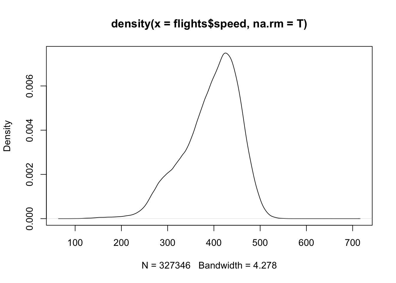
Now what happens if I do the following, will this work?
#plot(density(flights$speed))

#Unclear if we will have done ggplot at this point.
#ggplot(flights, mapping = aes(x = speed)) +
#  geom_density()
Nope! Why not?
Remember that dplyr verbs take a dataset and return a dataset, but unless we save the output nothing changes in our original dataset. We can overwrite flights with the result of our mutate command to actually save the new version that has this variable created:
flights <- mutate(flights,
       speed = distance/air_time*60)
And then we can graph the density:
ggplot(flights, mapping = aes(x = speed)) +
  geom_density()
#> Warning: Removed 9430 rows containing non-finite outside the scale
#> range (`stat_density()`).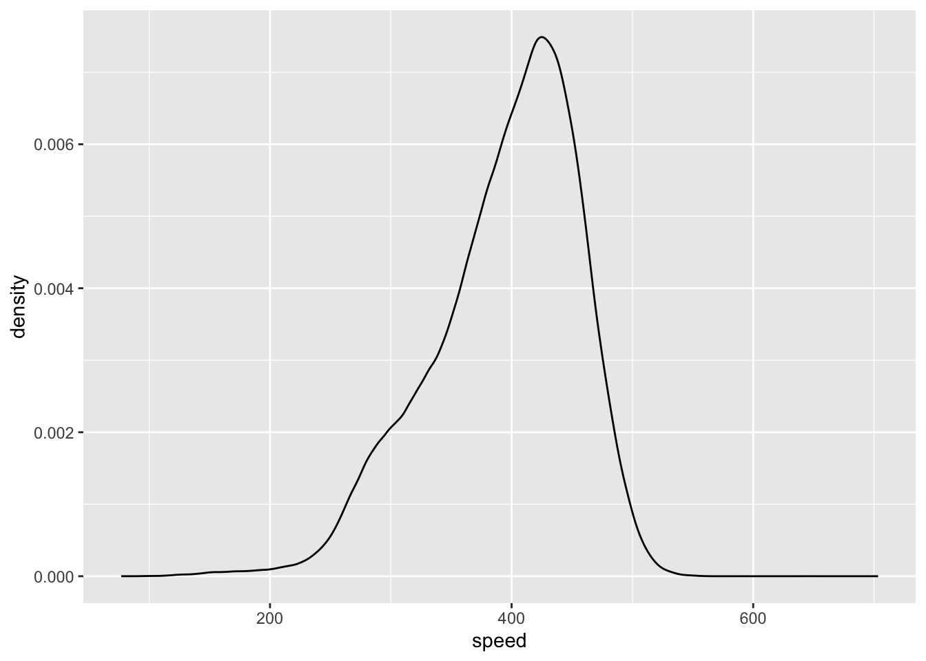
Another thing we might want to do with columns is to remove some. Like in base R, we think of this less as removing columns and more as keeping columns we want, via the select() function:
select(flights, year, month, day)
#> # A tibble: 336,776 × 3
#>     year month   day
#>    <int> <int> <int>
#>  1  2013     1     1
#>  2  2013     1     1
#>  3  2013     1     1
#>  4  2013     1     1
#>  5  2013     1     1
#>  6  2013     1     1
#>  7  2013     1     1
#>  8  2013     1     1
#>  9  2013     1     1
#> 10  2013     1     1
#> # ℹ 336,766 more rows
If we want to select all columns between two:
select(flights, year:day)
#> # A tibble: 336,776 × 3
#>     year month   day
#>    <int> <int> <int>
#>  1  2013     1     1
#>  2  2013     1     1
#>  3  2013     1     1
#>  4  2013     1     1
#>  5  2013     1     1
#>  6  2013     1     1
#>  7  2013     1     1
#>  8  2013     1     1
#>  9  2013     1     1
#> 10  2013     1     1
#> # ℹ 336,766 more rows
Or select all columns that are a certain class:
select(flights, where(is.character))
#> # A tibble: 336,776 × 4
#>    carrier tailnum origin dest
#>    <chr>   <chr>   <chr>  <chr>
#>  1 UA      N14228  EWR    IAH
#>  2 UA      N24211  LGA    IAH
#>  3 AA      N619AA  JFK    MIA
#>  4 B6      N804JB  JFK    BQN
#>  5 DL      N668DN  LGA    ATL
#>  6 UA      N39463  EWR    ORD
#>  7 B6      N516JB  EWR    FLL
#>  8 EV      N829AS  LGA    IAD
#>  9 B6      N593JB  JFK    MCO
#> 10 AA      N3ALAA  LGA    ORD
#> # ℹ 336,766 more rows
We can also not-select a variable. In otherwords getting everything except that variable.
select(flights, -year)
#> # A tibble: 336,776 × 20
#>    month   day dep_time sched_dep_time dep_delay arr_time
#>    <int> <int>    <int>          <int>     <dbl>    <int>
#>  1     1     1      517            515         2      830
#>  2     1     1      533            529         4      850
#>  3     1     1      542            540         2      923
#>  4     1     1      544            545        -1     1004
#>  5     1     1      554            600        -6      812
#>  6     1     1      554            558        -4      740
#>  7     1     1      555            600        -5      913
#>  8     1     1      557            600        -3      709
#>  9     1     1      557            600        -3      838
#> 10     1     1      558            600        -2      753
#> # ℹ 336,766 more rows
#> # ℹ 14 more variables: sched_arr_time <int>,
#> #   arr_delay <dbl>, carrier <chr>, flight <int>,
#> #   tailnum <chr>, origin <chr>, dest <chr>,
#> #   air_time <dbl>, distance <dbl>, hour <dbl>,
#> #   minute <dbl>, time_hour <dttm>, speed_old <dbl>,
#> #   speed <dbl>
Other helpful things to put in select:
-
starts_with("abc"): matches names that begin with “abc”.
select(flights, starts_with("dep"))
#> # A tibble: 336,776 × 2
#>    dep_time dep_delay
#>       <int>     <dbl>
#>  1      517         2
#>  2      533         4
#>  3      542         2
#>  4      544        -1
#>  5      554        -6
#>  6      554        -4
#>  7      555        -5
#>  8      557        -3
#>  9      557        -3
#> 10      558        -2
#> # ℹ 336,766 more rows-
ends_with("xyz"): matches names that end with “xyz”.
select(flights, ends_with("time"))
#> # A tibble: 336,776 × 5
#>    dep_time sched_dep_time arr_time sched_arr_time air_time
#>       <int>          <int>    <int>          <int>    <dbl>
#>  1      517            515      830            819      227
#>  2      533            529      850            830      227
#>  3      542            540      923            850      160
#>  4      544            545     1004           1022      183
#>  5      554            600      812            837      116
#>  6      554            558      740            728      150
#>  7      555            600      913            854      158
#>  8      557            600      709            723       53
#>  9      557            600      838            846      140
#> 10      558            600      753            745      138
#> # ℹ 336,766 more rows-
contains("ijk"): matches names that contain “ijk”.
select(flights, contains("dep"))
#> # A tibble: 336,776 × 3
#>    dep_time sched_dep_time dep_delay
#>       <int>          <int>     <dbl>
#>  1      517            515         2
#>  2      533            529         4
#>  3      542            540         2
#>  4      544            545        -1
#>  5      554            600        -6
#>  6      554            558        -4
#>  7      555            600        -5
#>  8      557            600        -3
#>  9      557            600        -3
#> 10      558            600        -2
#> # ℹ 336,766 more rows
Finally if we wish to rename variables we can use the rename verb. The argument you give rename is “new.name=old.name”. For some reason I always want this to be the other way around, so it takes some getting used to
flight <- rename(flights,
       tail.num = tailnum,
       speed.other = speed_old)
names(flights)
#>  [1] "year"           "month"          "day"
#>  [4] "dep_time"       "sched_dep_time" "dep_delay"
#>  [7] "arr_time"       "sched_arr_time" "arr_delay"
#> [10] "carrier"        "flight"         "tailnum"
#> [13] "origin"         "dest"           "air_time"
#> [16] "distance"       "hour"           "minute"
#> [19] "time_hour"      "speed_old"      "speed"
Again, we have not saved this renaming until we save a new dataset from the output.
Finally, relocate() allows us to move columns around in the dataset. By defualt, relocate moves things to be in the front of the dataset:
relocate(flights, time_hour)
#> # A tibble: 336,776 × 21
#>    time_hour            year month   day dep_time
#>    <dttm>              <int> <int> <int>    <int>
#>  1 2013-01-01 05:00:00  2013     1     1      517
#>  2 2013-01-01 05:00:00  2013     1     1      533
#>  3 2013-01-01 05:00:00  2013     1     1      542
#>  4 2013-01-01 05:00:00  2013     1     1      544
#>  5 2013-01-01 06:00:00  2013     1     1      554
#>  6 2013-01-01 05:00:00  2013     1     1      554
#>  7 2013-01-01 06:00:00  2013     1     1      555
#>  8 2013-01-01 06:00:00  2013     1     1      557
#>  9 2013-01-01 06:00:00  2013     1     1      557
#> 10 2013-01-01 06:00:00  2013     1     1      558
#> # ℹ 336,766 more rows
#> # ℹ 16 more variables: sched_dep_time <int>,
#> #   dep_delay <dbl>, arr_time <int>, sched_arr_time <int>,
#> #   arr_delay <dbl>, carrier <chr>, flight <int>,
#> #   tailnum <chr>, origin <chr>, dest <chr>,
#> #   air_time <dbl>, distance <dbl>, hour <dbl>,
#> #   minute <dbl>, speed_old <dbl>, speed <dbl>
But we can also specify using the .before and .after options:
relocate(flights, year:dep_time, .after = time_hour)
#> # A tibble: 336,776 × 21
#>    sched_dep_time dep_delay arr_time sched_arr_time
#>             <int>     <dbl>    <int>          <int>
#>  1            515         2      830            819
#>  2            529         4      850            830
#>  3            540         2      923            850
#>  4            545        -1     1004           1022
#>  5            600        -6      812            837
#>  6            558        -4      740            728
#>  7            600        -5      913            854
#>  8            600        -3      709            723
#>  9            600        -3      838            846
#> 10            600        -2      753            745
#> # ℹ 336,766 more rows
#> # ℹ 17 more variables: arr_delay <dbl>, carrier <chr>,
#> #   flight <int>, tailnum <chr>, origin <chr>, dest <chr>,
#> #   air_time <dbl>, distance <dbl>, hour <dbl>,
#> #   minute <dbl>, time_hour <dttm>, year <int>,
#> #   month <int>, day <int>, dep_time <int>,
#> #   speed_old <dbl>, speed <dbl>
relocate(flights, starts_with("arr"), .before = dep_time)
#> # A tibble: 336,776 × 21
#>     year month   day arr_time arr_delay dep_time
#>    <int> <int> <int>    <int>     <dbl>    <int>
#>  1  2013     1     1      830        11      517
#>  2  2013     1     1      850        20      533
#>  3  2013     1     1      923        33      542
#>  4  2013     1     1     1004       -18      544
#>  5  2013     1     1      812       -25      554
#>  6  2013     1     1      740        12      554
#>  7  2013     1     1      913        19      555
#>  8  2013     1     1      709       -14      557
#>  9  2013     1     1      838        -8      557
#> 10  2013     1     1      753         8      558
#> # ℹ 336,766 more rows
#> # ℹ 15 more variables: sched_dep_time <int>,
#> #   dep_delay <dbl>, sched_arr_time <int>, carrier <chr>,
#> #   flight <int>, tailnum <chr>, origin <chr>, dest <chr>,
#> #   air_time <dbl>, distance <dbl>, hour <dbl>,
#> #   minute <dbl>, time_hour <dttm>, speed_old <dbl>,
#> #   speed <dbl>
11.2 The pipe
So far it may seem that the “rules” of tidyverse/dplyr are pretty useless. Why do I need to create a whole new dataset just to rename a variable? The purpose for all of this comes together via the pipe operator.
Let’s try to answer this question. What are the fastest flights (in terms of mph) that arrive at Houston’s airport (IAH), identifying flights by their year, month, day, flight number, and departure airport?
To do this, we need to: filter down to IAH, create a speed variable, select only the variables we want, arrange the data so that fastest speed is at the top of the dataset.
To brush up, here is how we would do this in base R
library(nycflights13)
#Create new dataset
flights.base <- flights

#Create speed variable
flights.base$speed <- flights.base$distance/flights.base$air_time*60

#Filter to IAH
flights.houston <- flights.base[flights.base$dest=="IAH",]

#Select variables that we care about
flights.houston <- flights.houston[c("dest", "speed", "year","month", "day", "flight", "origin")]

#Re-order
flights.houston <- flights.houston[order(flights.houston$speed, decreasing = T),]

#View
head(flights.houston)
#> # A tibble: 6 × 7
#>   dest  speed  year month   day flight origin
#>   <chr> <dbl> <int> <int> <int>  <int> <chr>
#> 1 IAH    522.  2013     7     9    226 EWR
#> 2 IAH    521.  2013     8    27   1128 LGA
#> 3 IAH    519.  2013     8    28   1711 EWR
#> 4 IAH    519.  2013     8    28   1022 EWR
#> 5 IAH    515.  2013     6    11   1178 EWR
#> 6 IAH    515.  2013     8    27    333 EWR
OK, now let’s deploy our tidyr commands, remembering that each command outputs a dataframe that we have to save.
To do this, we need to: filter down to IAH, create a speed variable, select only the variables we want, arrange the data so that fastest speed is at the top of the variable.
library(tidyverse)
#Create new dataset
flights.tidy <- flights
#Filter to IAH
flights.tidy <- filter(flights.tidy, dest=="IAH")
#Create speed variable
flights.tidy <- mutate(flights.tidy, speed = distance/air_time*60)
#Select on the variables we are interested in
flights.tidy <- select(flights.tidy,dest,speed, year, month,day, flight, origin)
#Put the highest speed first
flights.tidy <- arrange(flights.tidy, desc(speed))
#View the datset
flights.tidy
#> # A tibble: 7,198 × 7
#>    dest  speed  year month   day flight origin
#>    <chr> <dbl> <int> <int> <int>  <int> <chr>
#>  1 IAH    522.  2013     7     9    226 EWR
#>  2 IAH    521.  2013     8    27   1128 LGA
#>  3 IAH    519.  2013     8    28   1711 EWR
#>  4 IAH    519.  2013     8    28   1022 EWR
#>  5 IAH    515.  2013     6    11   1178 EWR
#>  6 IAH    515.  2013     8    27    333 EWR
#>  7 IAH    515.  2013     8    27   1421 EWR
#>  8 IAH    515.  2013     8    27    302 EWR
#>  9 IAH    515.  2013     9    27    252 EWR
#> 10 IAH    515.  2013     8    28    559 LGA
#> # ℹ 7,188 more rows
OK that saved us some hassle in terms of quotation marks and square brackets, but it’s really not that much cleaner.
But, notice how in each command I am re-saving the same dataset and then putting that dataset back into the next command. What the pipe does it automatically sends the output of one command into the first argument of the next command. The pipe operator is |>. As such, we can re-write the above:
filter(flights,dest=="IAH") |>
mutate(speed = distance/air_time*60) |>
select(dest,speed, year, month,day, flight, origin) |>
arrange(desc(speed))
#> # A tibble: 7,198 × 7
#>    dest  speed  year month   day flight origin
#>    <chr> <dbl> <int> <int> <int>  <int> <chr>
#>  1 IAH    522.  2013     7     9    226 EWR
#>  2 IAH    521.  2013     8    27   1128 LGA
#>  3 IAH    519.  2013     8    28   1711 EWR
#>  4 IAH    519.  2013     8    28   1022 EWR
#>  5 IAH    515.  2013     6    11   1178 EWR
#>  6 IAH    515.  2013     8    27    333 EWR
#>  7 IAH    515.  2013     8    27   1421 EWR
#>  8 IAH    515.  2013     8    27    302 EWR
#>  9 IAH    515.  2013     9    27    252 EWR
#> 10 IAH    515.  2013     8    28    559 LGA
#> # ℹ 7,188 more rows
Notice here that I have only input the dataframe “flights” once, in the very first command. In all subsequent commands the pipe tells R to take the dataframe that is the output of one command and insert it as the dataframe for the next command.
One note: until recently the pipe operator was %>%. If you use the keyboard shortcut for the pipe: cmd+shift+m (on Apple) or ctrl+shift+m on PC, you will get this old pipe operator. The old operator still works fine and lots of people use it. I have updated to the new syntax that uses |>. If you want to as well, go to Tools>Global Options>Code and check the box for “Use native pipe operator”.
Note that the order really matters here. We could not do:
#select(flights, speed, time) |>
#  mutate(speed = distance/air_time*60)
Because we are trying to select the column “speed” before we have created it.
Right now the first line in our piped together command is filter(flights,dest=="IAH"). This works fine, but if we wanted to add a command before that one we would have to remember to take flights out of that command and put it in the new top level command. As such, it is better practice for your first command to be your dataset and then to pipe that into the first verb:
flights |>
  filter(dest=="IAH") |>
  mutate(speed = distance/air_time*60) |>
  select(dest,speed, year, month,day, flight, origin) |>
  arrange(desc(speed))
#> # A tibble: 7,198 × 7
#>    dest  speed  year month   day flight origin
#>    <chr> <dbl> <int> <int> <int>  <int> <chr>
#>  1 IAH    522.  2013     7     9    226 EWR
#>  2 IAH    521.  2013     8    27   1128 LGA
#>  3 IAH    519.  2013     8    28   1711 EWR
#>  4 IAH    519.  2013     8    28   1022 EWR
#>  5 IAH    515.  2013     6    11   1178 EWR
#>  6 IAH    515.  2013     8    27    333 EWR
#>  7 IAH    515.  2013     8    27   1421 EWR
#>  8 IAH    515.  2013     8    27    302 EWR
#>  9 IAH    515.  2013     9    27    252 EWR
#> 10 IAH    515.  2013     8    28    559 LGA
#> # ℹ 7,188 more rows
If we want to save this output we have to explicitly do so. Somewhat backwards, everything gets processed by dplyr left to right, but we put our save command right at the very beginning:
iah.speed <- flights |>
  filter(dest=="IAH") |>
  mutate(speed = distance/air_time*60) |>
  select(dest,speed, year, month,day, flight, origin) |>
  arrange(desc(speed))
IF IT IS HELPFUL, you can actually put the assignment operator at the very end, which I like doing because it follows the logical flow of the syntax. Dr. Pettigrew, who teaches PSCI 3800, hates that I do this. So you should probably avoid it.
flights |>
  filter(dest=="IAH") |>
  mutate(speed = distance/air_time*60) |>
  select(dest,speed, year, month,day, flight, origin) |>
  arrange(desc(speed)) -> iah.speed
Let’s do another example.
Display the tail numbers and destinations of all flights departing at La Guardia on April 1st that had a departure delay more than 100 minutes
11.3 Verbs that operate on groups
Another thing we have frequently done in R is to consider groups in the data, usually using a loop to calculate something group-by-group.
In the tidyverse we abandon loops because we can explicitly define groups and then execute commands based on those groups. If we use the verb group_by() we are telling R what groups we want to operator on:
flights |>
  group_by(month)
#> # A tibble: 336,776 × 21
#> # Groups:   month [12]
#>     year month   day dep_time sched_dep_time dep_delay
#>    <int> <int> <int>    <int>          <int>     <dbl>
#>  1  2013     1     1      517            515         2
#>  2  2013     1     1      533            529         4
#>  3  2013     1     1      542            540         2
#>  4  2013     1     1      544            545        -1
#>  5  2013     1     1      554            600        -6
#>  6  2013     1     1      554            558        -4
#>  7  2013     1     1      555            600        -5
#>  8  2013     1     1      557            600        -3
#>  9  2013     1     1      557            600        -3
#> 10  2013     1     1      558            600        -2
#> # ℹ 336,766 more rows
#> # ℹ 15 more variables: arr_time <int>,
#> #   sched_arr_time <int>, arr_delay <dbl>, carrier <chr>,
#> #   flight <int>, tailnum <chr>, origin <chr>, dest <chr>,
#> #   air_time <dbl>, distance <dbl>, hour <dbl>,
#> #   minute <dbl>, time_hour <dttm>, speed_old <dbl>,
#> #   speed <dbl>
Now this command doesn’t do anything, but notice that now it explicitly says that “groups” is set to month and that there are 12 groups. Now subsequent operations will automatically proceed by the group variable.
To actually do something we use the summarize() command, which automatically calculates things separately for each group. Note, the British/Canadian spelling summarise() also works and you may occasionally catch me using that.
So if we want to know the average departure delay by month it is as simple as:
flights |>
  group_by(month) |>
  summarize(avg.delay = mean(dep_delay,na.rm=T))
#> # A tibble: 12 × 2
#>    month avg.delay
#>    <int>     <dbl>
#>  1     1     10.0
#>  2     2     10.8
#>  3     3     13.2
#>  4     4     13.9
#>  5     5     13.0
#>  6     6     20.8
#>  7     7     21.7
#>  8     8     12.6
#>  9     9      6.72
#> 10    10      6.24
#> 11    11      5.44
#> 12    12     16.6
We can add additional lines to the summarize command to calculate more group means. One helpful command is n() which will simply give the counts by group.
flights |>
  group_by(month) |>
  summarize(avg.delay = mean(dep_delay,na.rm=T),
            obs = n(),
            range.delay = diff(range(dep_delay, na.rm=T)))
#> # A tibble: 12 × 4
#>    month avg.delay   obs range.delay
#>    <int>     <dbl> <int>       <dbl>
#>  1     1     10.0  27004        1331
#>  2     2     10.8  24951         886
#>  3     3     13.2  28834         936
#>  4     4     13.9  28330         981
#>  5     5     13.0  28796         902
#>  6     6     20.8  28243        1158
#>  7     7     21.7  29425        1027
#>  8     8     12.6  29327         546
#>  9     9      6.72 27574        1038
#> 10    10      6.24 28889         727
#> 11    11      5.44 27268         830
#> 12    12     16.6  28135         939
We can add multiple variables to the group_by() command and the groups will become unique combinations of those variables. So if we want the group to be a day of the year:
flights |>
  group_by(year, month,day)
#> # A tibble: 336,776 × 21
#> # Groups:   year, month, day [365]
#>     year month   day dep_time sched_dep_time dep_delay
#>    <int> <int> <int>    <int>          <int>     <dbl>
#>  1  2013     1     1      517            515         2
#>  2  2013     1     1      533            529         4
#>  3  2013     1     1      542            540         2
#>  4  2013     1     1      544            545        -1
#>  5  2013     1     1      554            600        -6
#>  6  2013     1     1      554            558        -4
#>  7  2013     1     1      555            600        -5
#>  8  2013     1     1      557            600        -3
#>  9  2013     1     1      557            600        -3
#> 10  2013     1     1      558            600        -2
#> # ℹ 336,766 more rows
#> # ℹ 15 more variables: arr_time <int>,
#> #   sched_arr_time <int>, arr_delay <dbl>, carrier <chr>,
#> #   flight <int>, tailnum <chr>, origin <chr>, dest <chr>,
#> #   air_time <dbl>, distance <dbl>, hour <dbl>,
#> #   minute <dbl>, time_hour <dttm>, speed_old <dbl>,
#> #   speed <dbl>
And then to figure out how many flights occur on each day:
daily <- flights |>
  group_by(year, month,day) %>%
  summarize(n = n(),
            avg.delay = mean(dep_delay, na.rm=T))
#> `summarise()` has grouped output by 'year', 'month'. You
#> can override using the `.groups` argument.
daily
#> # A tibble: 365 × 5
#> # Groups:   year, month [12]
#>     year month   day     n avg.delay
#>    <int> <int> <int> <int>     <dbl>
#>  1  2013     1     1   842     11.5
#>  2  2013     1     2   943     13.9
#>  3  2013     1     3   914     11.0
#>  4  2013     1     4   915      8.95
#>  5  2013     1     5   720      5.73
#>  6  2013     1     6   832      7.15
#>  7  2013     1     7   933      5.42
#>  8  2013     1     8   899      2.55
#>  9  2013     1     9   902      2.28
#> 10  2013     1    10   932      2.84
#> # ℹ 355 more rows
We have a new day level dataset that tells us information about those days. Note that by default the groups in this new dataset are year and month, but it’s possible to change that default behavior.
We can also just remove the group structure of the data. Say we want the average daily delay. If we try to run that on our dataset right now:
daily |>
  summarize(avg.daily.delay = mean(avg.delay))
#> `summarise()` has grouped output by 'year'. You can
#> override using the `.groups` argument.
#> # A tibble: 12 × 3
#> # Groups:   year [1]
#>     year month avg.daily.delay
#>    <int> <int>           <dbl>
#>  1  2013     1           10.0
#>  2  2013     2           11.1
#>  3  2013     3           13.6
#>  4  2013     4           13.9
#>  5  2013     5           13.2
#>  6  2013     6           20.9
#>  7  2013     7           21.8
#>  8  2013     8           12.6
#>  9  2013     9            6.92
#> 10  2013    10            6.19
#> 11  2013    11            5.30
#> 12  2013    12           16.9
It’s going to do it by year-month because that’s what the groups are set to right now. But if we use ungroup() we can get rid of that and do it for the whole dataset: