7 Review

Similar to the questions at the end of the chapters, knowledge of the contents of this review chapter is not necessarily sufficient to ensure success on the midterm. This summary is here as a reference guide to what we’ve covered, and allows me to emphasize the things that I find to be important.

7.1 Survey Research Basics

In the introduction I talked through a brief history of surveys, why they are so important, and how we have arrived at the modern paradigm of survey research.

In this chapter I will introduce more formally the nature of surveys and the framework we will use to look at the quality of surveys.

7.1.1 What is a survey?

A survey is a systematic method for gathering information from (a sample of) entities for the purposes of constructing quantitative descriptors of the attributes of a larger population of which the entities are members.

There are three key things here that are worth highlighting.

• Systematic. This is not just going out and interviewing people and compiling the result. To properly be a survey we must have a systematic process. A survey instrument that is identical. A sampling plan. A coding plan. A weighting plan. An analysis plan. All of this needs to be recorded, reported, and be able to be replicated.

• Quantitative. There are lots of questions that are best suited to qualitative analysis and deep interviews. But these things are not going to be treated as “surveys” in this framework. Here we are dealing with things that we can measure and perform math on. Things like proportions, means, correlations, and regressions.

• A sample of a population. To distinguish what we are doing from a census, in a survey we have a population of interest (say, all U.S. adults) and we use a sample of that population (say, 1000 randomly selected individuals) to infer information about that population.

7.1.2 Surveys from two perspectives

1. Survey Mode and Sampling Frame

2. Questionnaire Design and Sample Selection

3. Recruit and Measure Sample

4. Code and Edit Data

5. Make post-survey adjustments

6. Perform Analysis

1. Validity

2. Measurement Error

3. Processing Error

4. Coverage Error

5. Sampling Error

6. Non-Response Error

7. Adjustment Error

7.1.3 Total Survey Error (TSE)

Taken overall, the two sides of the figure represent the “Total Survey Error” (TSE) paradigm. As mentioned above, when we report the margin of error in a survey we are only talking about sampling error. Just one of the many possible sources of error. We report this one because it is a known quantity, and we cannot measure any of the others.

7.2 Questionnaire Design

We want to think about how the construct turns into the measure which turns into the response, and any differences that occur during these processes.

Mathematically, we can think about the response being a function of the underlying construct and some amount of “validity error”:

\[ Y_i = \mu_i + \epsilon_i \]

Where \(\epsilon_i\) is the validity error for an individual: how much (and in what direction) their true measured value deviates from their true construct value.

They then respond to the question, which is subject to measurement error:

\[ y_{it} = Y_i + u_{it} \]

Where \(u_{it}\) is how much the response for individual \(i\) at time \(t\) varies from their true measurement value.

We can combine these two equations, subbing in the left hand side in equation 1 for the \(Y_i\) in equation 2 to get:

\[ y_{it} = \mu_i + \epsilon_i + u_{it} \]

Whereby the individual’s response is a function of their true underlying value, validity error, and measurement error.

7.2.1 Validity

“Validity” simply means a measure that has a minimal difference between the response and the value of the construct.

Specifically, we are interested in:

\[ y_{it}-\mu_i \to 0 \]

The difference between the measure and the construct to approach zero. Now this is for the individual, when we think about a measure having validity for everyone, we think about the correlation of \(y_{it}\) and \(\mu_i\). A measure is valid when there is a high correlation between people’s measured values and their construct values:

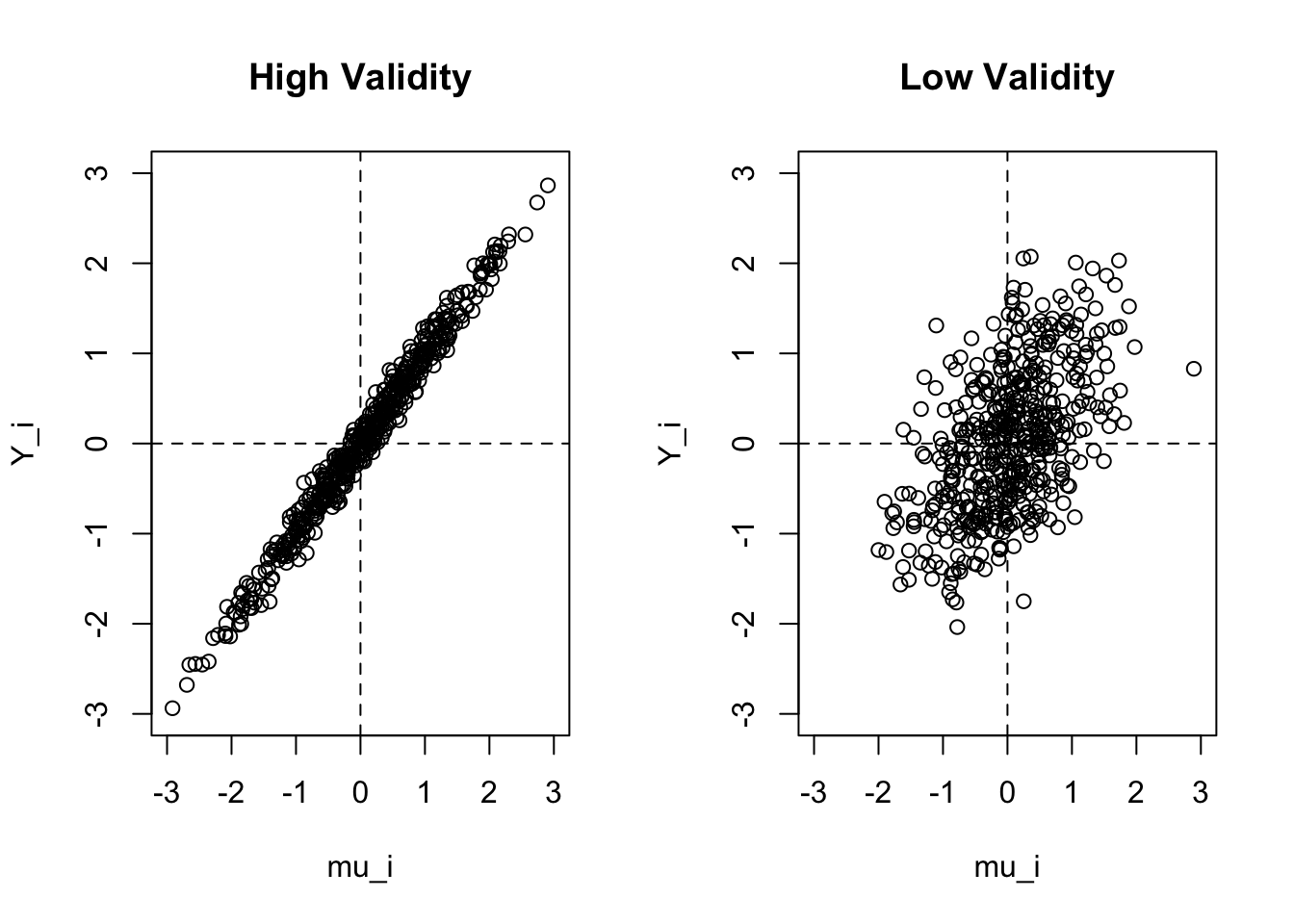
Why might a measure have low validity? Because we are looking at the actual response, low validity can appear as a function of either “validity error” \(\epsilon_i\) or “measurement error” \(u_{it}\).

There will be validity error when the measure itself doesn’t do a good job of matching the construct.

Measurement error would be a situation where people’s true answer to the question is the same as the construct but their actual recorded response differs.

How to assess validity?

The first, and simplest is face validity. This is simply: would people (your respondents, other experts) think that the question is measuring the construct?

A related concept is Content Validity. This similarly involves qualititatively assesing questions, but rather than an informal “does this seem right?”, it focuses more on whether subject experts believe that the question covers all relevant dimensions.

A more statistical way to assess validity is through Convergent Validity. Here we are interested if a measure of correlates highly with other measures of the same construct.

An opposite approach is to look at Divergent Validity, which is where we look at the responses across groups of people for whom we expect differences.

7.2.2 Reliability

The second aspect of question quality that we are interested in is Reliability. While validity looked at the degree to which a single response varied from the construct of interest (\(y_{it} - \mu_i=0\)?), reliability focuses on how much individual responses vary from each other over repeated measurements.

We want to know how much that measurement error differs over repeated trials:

\[ Var(u_{i1},u_{i2},u_{i3}, \dots u_{it}) = Var(u_{it}) \]

A measure is unreliable if people’s answers change on it to a high degree in repeated measures even though their underlying value of \(Y_i\) hasn’t changed.

7.2.3 The Psychology of Question Answering

1.Comprehension

In short, the respondent will be sub-conciously trying to understand what the point of the question is. This includes parsing the working of the question, assigning meaning to the various elements in the question, determining the range of permissible answers, and attempting to infer the purpose behind the question.

3. Retrieval

4. Estimation and Judgement

For factual questions if the respondent doesn’t have an immediate answer they have to process the thoughts and memories they are able to access in order to produce an answer.

For attitudes the process is different. We will cover this extensively through the Zaller and Feldman reading, but in general we do not believe that people walk around with attitudes “ready to go” in their heads, but instead construct them on the fly.

4. Reporting

Finally, after comprehending the question, accessing memories, and processing those memories, the respondent is ready to report an answer. Critically here they have to fit their desired answer to the response options that are presented.

7.2.4 Alternative Routes to an Answer

A critical alternative route to know is satisficing, as opposed to optimizing.

A satisficer has as their goal to provide a “reasonable” answer in as quick of time as possible with as little cognitive demands as possible.

7.2.5 Problems in Answering Survey Questions

1. Problems in encoding

The respondent simply may not have put what you care about into long term memory.

2. Problems interpreting the question.

Respondent’s may have more difficulty than you imagine understanding what you are asking in the question, and may try to read extra context into words in a way that you would not expect. Includes faulty presupposition and over-interpreting the question.

3. Problems with memory

In problem number (1) we discusssed issues where people did not encode the thing you are asking for in the first place. This problem is a more general one where they have the memory but the question that we ask does not lead them to actually generating that information. Groves splits this into 4 sub-parts.

4. Problems in estimation.

For both attitudinal and behavioral questions some respondents may have a precise answer readily accessible, but others will have to “construct” their answers on the fly which can lead to error. Impression based estimation very susceptible the response options offered.

5. Errors in judgement for attitudinal questions.

Zaller and Feldman.

6. Errors in formatting an answer.

Open vs closed response scales. For closed response scales people are susceptible to being influenced by the numbers you provide. People can get overwhelemd when too many options, but feel left out by too few.

7. Motivated misreporting.

For sensitive questions an additional problem is people mis-reporting their answers on purpose. Think expansively about this! Not just illegal and amoral behavior, but also strong norms in politics of how people “should” act.

8. Navigational errors

Not much of a problem.

7.2.6 Guidelines for Writing Good Questions

7.2.6.1 Non-sensitive questions about behavior

1. With closed questions, include all reasonable possibilities as explicit response options.

2. Make the questions as specific as possible.

3. Use words that virtually all respondents will understand.

4. Lengthen the questions by adding memory cues to improve recall.

5. When forgetting is likely, use aided recall.

6. When the evens of interest are frequent but not very involving, have respondents keep a diary.

7. When long recall periods must be used, us a life event calendar to improve reporting.

8. To reduce telescoping errors (misdating events), ask respondents to use household records or use bounded recall (give them their previous answer).

9. If cost is a factor, consider whether proxies might be able to provide accurate information. (ex. use parents to gain information about children, rather than interviewing children.)

7.2.6.2 Sensitive questions about behavior

1. Use open rather than closed questions for eliciting the frequency of sensitive behaviors.

2. Use long rather than short questions.

3. Use familiar words in describing sensitive behaviors.

4. Deliberately load the question to reduce misreporting.

5. Ask about long periods or periods from the distant past first in asking about sensitive behaviors.

6. Embed the sensitive question among other sensitive items to make it stand out less.

7. Use self administered mode.

8. Consider a diary.

9. Include additional items to assess how sensitive the behavioral questions were.

10. Collect validation data.

7.2.6.3 Attitude Questions

In political surveys we care much more about attitude questions, so we will spend a bit more time here.

1. Specify the attitude object clearly.

2. Avoid double-barreled questions.

3. Measure the strength of the attitude.

4. Use bipolar items except when they might miss key information.

5. Carefully consider which alternatives to include.

6. In measuring change over time, ask the same question each time.

7. When asking general and specific questions about a topic, ask the general question first.

8. When asking about multiple items, start with the least popular.

9. Use closed questions for measuring attitudes.

10. Use 5-7 point response scales and label every point.

11. Start with the end of the scale that is the least popular.

12. Use analogue devices like thermometers to collect more detailed information.

13. Use ranking only if the respondent can see all the alternatives.

14. Get ratings for every item of interest, do not use check all that apply.

7.2.7 Zaller and Feldman: A Simple Theory of the Survey Response

Two empirical facts:

The reliability of attitude questions is very low.

The other type of “error” that occurs is response effects, which are systematic variance that comes from people answering questions differently under different circumstances.

The theory forwarded to fit these things is that people have stored in their long term working memory a high number of considerations about important issues that may or may not conflict with one another. When we say that an opinion is “constructed” in real time, what we are saying is that people pull some of these considerations out in response to the question, and the nature and balance of those considerations may change at different times and under different circumstances.

1. Ambivalence: Most people possess opposing considerations on most issues.

2. Response: Individuals answer survey questions by averaging across the considerations that happen to be salient at the moment of response.

3. Accessibility: A stochastic (random) process where considerations that have been recently thought about are somewhat more likely to be sampled.

7.2.8 Perez

The considerations that we have are not just isolated things floating around in our long term memories. Instead, we think that considerations are linked together in a “lattice like” network. When you access one consideration you are more likely to also pull out the ones that are closely associated with it. Considerations become linked when they are thought of together often, or when they are initially encoded together. Language effects come in through the effect of encoding different pieces of information has on their accessibility.

The results indicate that individuals who took the survey in English have higher political knowledge, and that is specifically driven by having higher knowledge of traditional “American” political facts. Further, these individuals report having a higher Latino identity than those who interviewed in spanish. This might seem odd at first, but this is what is predicted because the categorization of “Latino” only makes sense in the American context. Those interviewed in spanish are less likely to think of themselves as Latino and more likely to associate themselves with their country of origin.

7.3 Sampling

This section will talk more about moving from a target population to a sampling frame to a sample, and the errors that can occur through that process.

The actual units that we wish to sample in this framework are called “elements”. This is more complicated then “who are we talking to”.

The universe of all the elements that we wish to study is the “population”.

The “sampling frame” is the real list or process that tries to contain every element in the population. This is not the sample itself, but an enumeration of all of the population.

The fundamental thing that you need to know is this: your sampling frame ideally gives every element in the population a known and non-zero probability of being selected.

7.3.1 Under Coverage

The most extreme case of breaking this tenet is “under-coverage” which is the case when there are elements of the population that are not in your sampling frame at all. In this case their probability of being selected into the sample is now zero.

Coverage error survey can (theoretically!) be calculated through the formula:

\[ Cov.Error = \frac{U}{N}(\bar{Y_c} - \bar{Y_u}) \]

Where \(U\) is the total number of uncovered people, \(N\) is the total number of people in the population, \(\bar{Y_c}\) is the value for the variable we are studying for the people who are in the sampling frame, and \(\bar{Y_u}\) is the value of the variable for the people who are not in the sampling frame.

To put a finer point on this: we only care about under-coverage if the opinions of those not covered are systematically different than those who are covered.

7.3.2 Inelegible units

The opposite problem occurs when there are elements in our sampling frame who should not be there. Similar to the above, we only really care about this if these people have systematically different opinions then the eligible people, and would therefore bias the results.

7.3.3 Complicated non-zero probabilities

In some surveys there can be some complicated probabilities associated with the sampling frame that need to be adjusted for.

Let’s say you have 10000 houses in your sampling frame, which represents an unknown number of actual people (the elements), and you wish to sample 1000 people.

If you call (or mail!) a household with 2 people in it and one person is randomly selected to fill out the survey, then that person had a \(\frac{1}{1000}*\frac{1}{2} = \frac{1}{2000}\) probability of being selected into the survey.

Consider a second household with 5 people in it, one of whom is similarly randomly selected to fill in the survey. That person had a \(\frac{1}{1000}*\frac{1}{5} = \frac{1}{5000}\) probability of being selected into the survey.

People in smaller houses therefore have a higher a priori probability of being included in the survey then people in larger houses. If people who live in houses with more people have systematically different opinions than people who live in houses with less people, then not correcting for this will give you a biased estimate.

7.3.4 Sampling Error for Simple Random Samples

When you read a poll release on a news website it will say something like “These results accurate to plus or minus 2.1 percentage points, 19 times out of 20”, or “The margin of error of this poll is plus or minus 2.1 percentage points.”

At the conclusion of this section you will understand exactly how these numbers are arrived at.

Actually: I can just tell you exactly how these numbers are arrived at.

The margin of error of a poll is determined by:

\[ MOE = 1.96 * \sqrt{\frac{.25}{n}} \]

Where \(n\) is the number of people in a poll. If there are 2177 people in a poll then:

1.96*sqrt(.25/2177)
#> [1] 0.02100375

The margin of error is plus or minus 2.1 percentage points.

You should understand where each of the numbers in the equation for the MOE come from.

If the truth in the population is that 50% of people believe something and we repeatedly took samples of 1000 people and calcualted the sample mean in each of those samples, we believe that the resulting sampling distribution would look like this:

x <- seq(.4,.6,.001)

plot(x, dnorm(x, mean = .5, sd = sqrt(.25/1000)), type="l", main="Sampling Distribution",
     xlab="",ylab="Density")

A normal distribution centered on the true population value (50%), with a standard error (the standard deviation of the sampling distribution) of \(\sqrt{\frac{.25}{n}}\), where .25 is the variance of a Bernoulli random variable where the probability of success is 50% (\(V[bern] = \pi*(1-\pi) = .5*.5 = .25\)).

The area that contains 95% of the probability mass symmetrical around the mean in this distribution is plue or minus 1.96 standard errors away from the mean:

#high
high <- .5 + 1.96*sqrt(.25/1000)
low <- .5 - 1.96*sqrt(.25/1000)
high
#> [1] 0.5309903
low
#> [1] 0.4690097
plot(x, dnorm(x, mean = .5, sd = sqrt(.25/1000)), type="l", main="Sampling Distribution",
     xlab="",ylab="Density")
abline(v=high, lty=2)
abline(v=low, lty=2)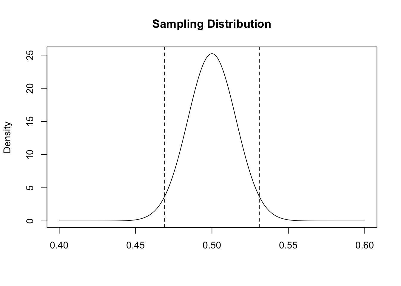

Confirm this with R’s built in calculus tools:

qnorm(.975, mean = .5, sd = sqrt(.25/1000))
#> [1] 0.5309898
qnorm(.025, mean = .5, sd = sqrt(.25/1000))
#> [1] 0.4690102

The central limit theorem is what provides us the equation for the standard error, and tells us that the sampling distribution gets skinnier when our n gets larger. This makes good theoretical sense because what we know about the law of large numbers. For any given sample, the larger the sample the more likely the sample mean will equal the population truth. Therefore for a larger n all possible samples will be expected to be closer to the truth than for any smaller n. 

The margin of error is a 95% confidence interval. When we place a correctly sized sampling distribution around our sample mean, similarly calculating the area that contains 95% of the probability mass (again, plus or minus 1.96 standard errors) creates an area that will contain the true population proportion 95% of the time.

The central limit theorem tells us that the standard error is \(\sqrt{\frac{V[X]}{n}}\). Because in survey research we are almost always dealing with proportions, we can replace the numerator of this equation with the variance of a bernoulli random variable, which is the probability of success multiplied by the probability of failure: \(\sqrt{\frac{\pi*(1-\pi)}{n}}\). In survey research (and all science) we like to bias against false positives (saying something is real when it’s not) so it is convention in survey research to set \(\pi\) to .5 for this equation, because that makes the numerator as large as possible, \(se=\sqrt{\frac{.5*.5}{n}} =\sqrt{\frac{.25}{n}}\).

Remember that this margin of error only represents the error in our poll that is due to random sampling, it does not take into account measurement error, non-coverage error, processing error etc.

Still, this provides a reasonable baseline of what we can expect the error to be for a poll of the size that we are doing.

It’s also important to remember that this is the margin of error around each proportion in the survey. If we are comparing two proportions each of those has a margin of error.

7.3.5 Finite Population Corrections

One of the hallmarks of the central limit theorem is that it operates well regardless of the size of the population from which you are sampling from.

For example, the standard error for a poll of 1000 people from a population of 1 million people should have a standard error of \(\sqrt{\frac{.25}{1000}} = 0.016\):

pop <- rbinom(1E6, 1, .5)
means <- NA

for(i in 1:10000){
  means[i] <- mean(sample(pop, 1000))
}
sd(means)
#> [1] 0.01563311

And the same is true for a poll of 1000 people from a population of 100 million people:

pop <- rbinom(1E8, 1, .5)
means <- NA

for(i in 1:10000){
  means[i] <- mean(sample(pop, 1000))
}
sd(means)
#> [1] 0.0159657

This is why we can use the same sized sample to study Canada, the US, and China.

But surely this logic breaks down eventually. If we have a population of 1001 people and do a survey of 1000 people our standard error is not going to be .016:

pop <- rbinom(1001, 1, .5)
means <- NA

for(i in 1:10000){
  means[i] <- mean(sample(pop, 1000))
}
sd(means)
#> [1] 0.0005000106

Way smaller!

We can mathematically determine finite population correction whenever our sample size approaches the populationsize. To get the correct margin of error we can calculate the standard error with a correction factor:

\[ \sqrt{\frac{N-n}{N-1}} *\sqrt{\frac{.25}{n}} \]

Where \(N\) is the size of the population and \(n\) is the sample size.

So for a case where we have a population of 1001 and a sample size of 1000:

\[ SE_{f} = \sqrt{\frac{1001-1000}{1001-1}} *\sqrt{\frac{.25}{1000}}\\ SE_{f} = \sqrt{\frac{1}{1000}} *0.016\\ SE_{f} = .0005 \]

Here is what the correction looks like for a sample size of 1000 at different population levels. (Note the non-linear x-axis)

pop <- 10^seq(3,7,0.1)

correction <- sqrt((pop-1000)/(pop-1))

plot(log10(pop), correction, axes=F, pch=16, 
     xlab="Population Size", 
     ylab="Finite Population Correction")
axis(side=1, at = 3:7, labels = 10^(3:7), )
axis(side=2, las=2)
abline(h=1, lty=2, col="firebrick")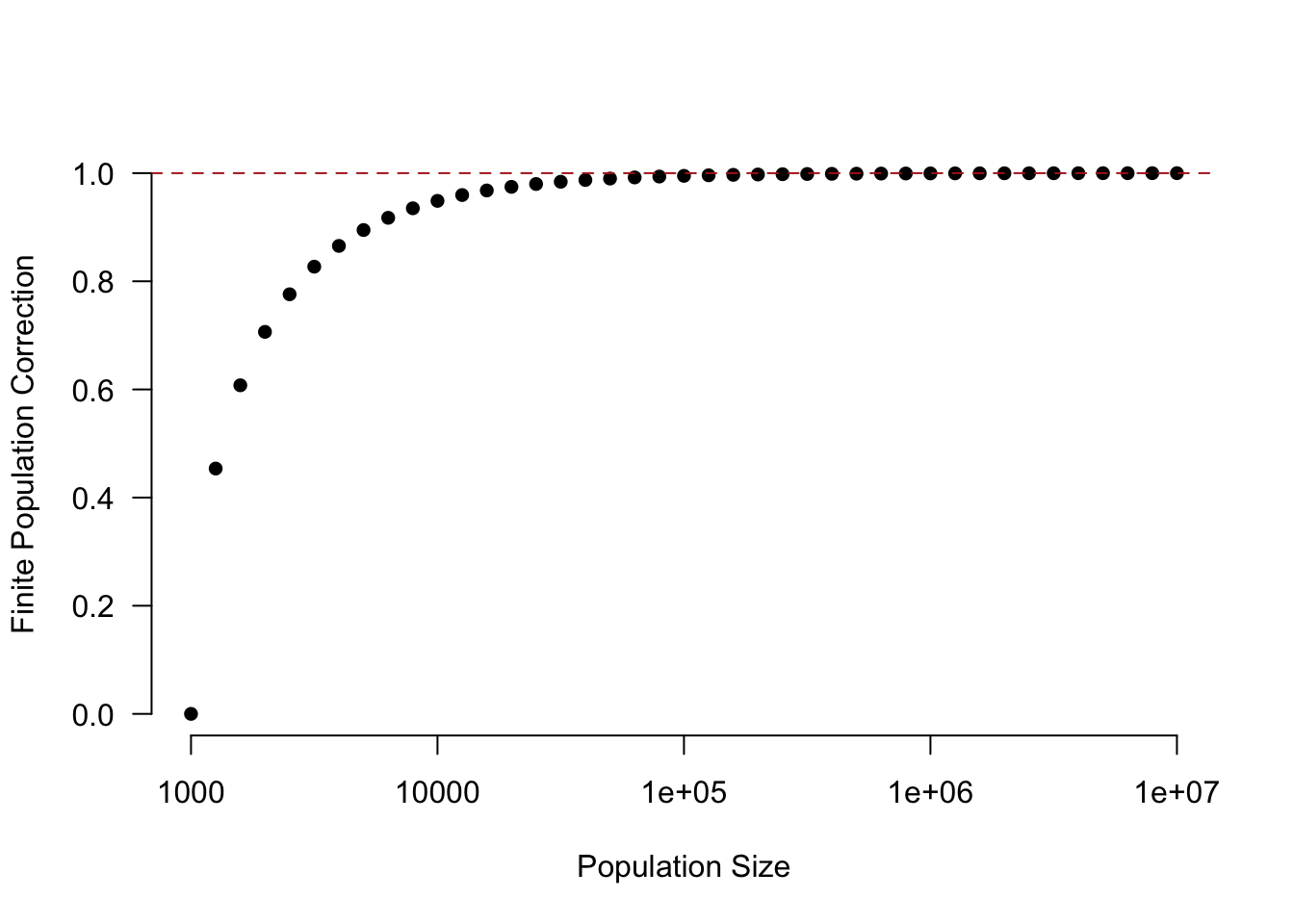

7.3.6 The 1936 Literary Digest Poll

The question taken on by these article is the degree to which this polling error was a consequence of coverage error of non-response error.

Helpfully, Gallup was also polling during this time period (in a more systematic, but also flawed way). And in their poll they asked three key questions:

1. Do you own a phone/car?

2. Did you receive a Literary Digest ballot?

3. Did you send it in?

Remember that coverage error occurs when the people who are in the sampling frame have systematically different opinions than those people that are not in the sampling frame.

We can’t see the sampling frame directly here – but we know that Literary Digest used car registration lists and telephone books, which means that people without a car and phone were less likely to be covered by the poll.

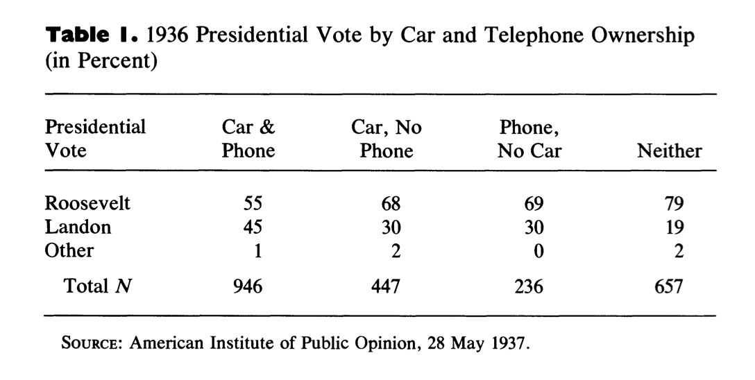
The first table looks at vote choice by these two variables. As the article discusses, because this poll was taken after the election, we expect that all of these numbers are probably a bit too high for Roosevelt. There is (or was, it’s probably less prevalent now) a consistent “winners effect” in post election polls where more people recall or report voting for the winning candidate than really did. Regardless, in every category Roosevelt, not Landon, is the preferred candidate. This is the first clue that it’s not just coverage error that caused the polling miss. For that to be the case there would have to be at least some group here who preferred Landon or Roosevelt. However, we do see that as someone is less likely to be in the sampling frame (not owning either a car or phone) they are more likely to support FDR. This is evidence that the people not in the samplign frame had different opinions (more pro FDR) than those in the sampling frame.

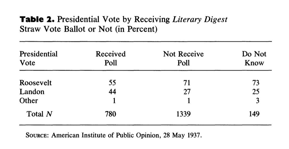
The second important question gets at the coverage issue in a more direct way. Because Literary Digest sent a postcard to nearly everyone in the sampling frame, simply asking if they got one is another look into the sampling frame. This might be a preferable question because we are asking people directly, but it might also suffer due to people forgetting whether they got a postcard or not.

This question shows relatively similar results. People who did not receive the LD poll (and therefore were not in the sampling frame) were more pro FDR than people who did receive the poll.

But these coverage issues alone are not enough to explain the polling miss. To do so we need to preview our next topic, which is non-response. Non-response bias occurs when their is correlation between responding to the poll and the question of interest (here vote choice). So in this third table we see, among those who received a ballot, whether there was a difference in opinion towards the candidates.

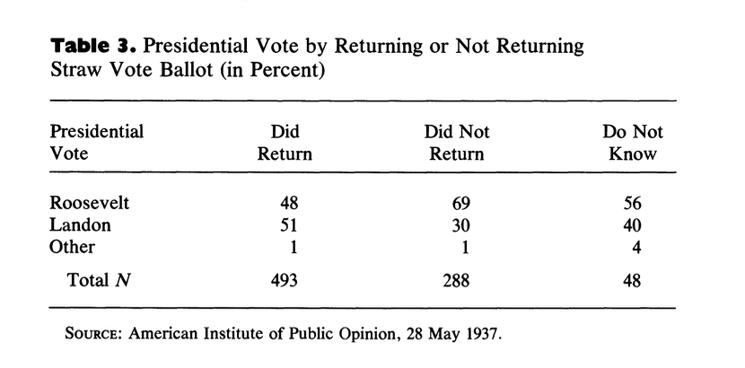
What we see is that the people who returend a ballot were far more likely to support Landon, and the people who did not return a ballot were far more likely to support Roosevelt. This indicates non-response bias was a significant contributor to the problem.

To sum this up: if everyone who was sent a ballot returned in the poll still would have been biased (that’s coverage error). And if everyone had been sent a ballot the poll still would have been biased (that’s non-response error). But both of these things happened at once, creating the huge error that brought down Literary Digest.