x <- seq(0,10)
plot(x, dbinom(x,10, prob=.5))
abline(v=7, lty=2)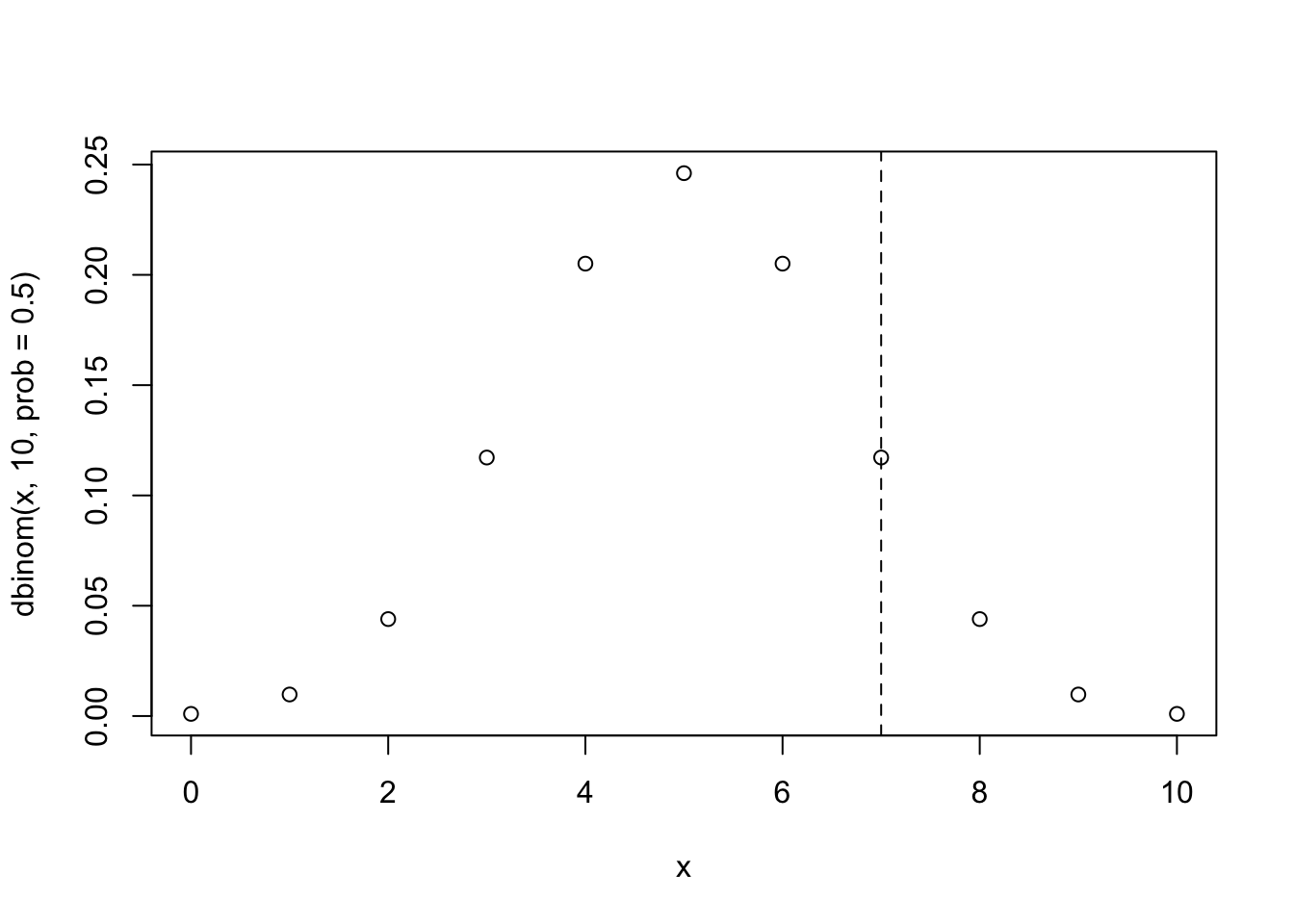
📄 Download the R code from this chapter
📝 Download the class handout for this chapter
We have spent this entire course learning how to make inferences about populations from samples of data. Every tool we have built – confidence intervals, hypothesis tests, standard errors – follows the same fundamental logic. We consider our test statistic to be drawn from a random variable (the sampling distribution) that has a known shape. We posit something about that sampling distribution (that it is centered on 50% for a poll, or on 0 for the difference in means, or whatever we want), and then ask: how surprising is our test statistic given our assumption?
This approach to statistics is called frequentist statistics. It is so called because the sampling distribution describes the hypothetical distribution of all possible test statistics if we estimated them in many samples. This is the dominant paradigm in the social sciences, and everything you have learned in this course falls under that umbrella. But it is not the only way to think about uncertainty. In this chapter we are going to explore an alternative: Bayesian statistics.
This chapter is not going to make you a Bayesian statistician. That would take a whole other course (or two). What I want to do is give you an intuition for how Bayesian reasoning works, show you how it differs from what we’ve been doing, and let you see that the two approaches are answering fundamentally different questions. Whether one is “better” than the other is a debate that has been raging for decades and I am not going to settle it here. But I think understanding both makes you a better consumer of statistics regardless of which camp you end up in.
Let’s think through how we have been thinking about hypothesis testing so far. We have some sample of data, and we ask:
Frequentist question: If the null hypothesis is true, how likely are these data?
We calculate a p-value, which is the probability of observing data as extreme or more extreme than what we got, assuming the null is true. If that probability is small enough (below our \(\alpha\) threshold), we reject the null.
Bayesian statistics flips this around entirely. Instead of asking how likely the data are given some hypothesis, a Bayesian asks:
Bayesian question: Given the data I have observed, how likely is the hypothesis?
Read those two questions again. They are not the same question. This is a point that trips up a lot of people – including a lot of professional researchers. When we calculate a p-value of 0.03, we are not saying there is a 3% chance the null hypothesis is true. We are saying there is a 3% chance of seeing data this extreme if the null were true. Those are very different statements.
The Bayesian approach gives you something that, frankly, most people think frequentist statistics gives them: a direct probability statement about the hypothesis. “There is an 85% probability that the true effect is positive.” “There is a 94% probability that Candidate A is ahead.” These are Bayesian statements. You cannot make them in the frequentist framework – even though people do it all the time without realizing they are breaking the rules.
The center of Bayesian statistics is Bayes theorem. The good news is that we can derive this equation completely with the tools we built in the probability section at the start of the semester.
The conditional probability of A given B is equal to:
\[P(A|B) = \frac{P(A \& B)}{P(B)}\]
The probability of A and B both occurring divided by the probability of B occurring alone.
Likewise we could write out:
\[ \begin{aligned} P(B|A) &= \frac{P(B \& A)}{P(A)}\\ P(A\&B) &= P(B|A)*P(A) \end{aligned} \]
Subbing in what we just showed for \(P(A\&B)\) we get Bayes’ Theorem:
\[P(A|B) = \frac{P(B|A) \times P(A)}{P(B)}\]
That’s great that the math gives us that answer, but why is this an important formula?
Here is the most basic sort of problem we can think about using Bayes theory:
Let’s say you take a medical test for a disease and get a positive result. Given that every test has a potential for false positives (saying you have the disease when you don’t), how can we think about the probability you have the disease (A), given that you have a positive test (B).
Subbing those things in:
\[P(Disease|Pos) = \frac{P(Pos|Disease) \times P(Disease)}{P(Pos)}\]
Let’s take each of these things in turn.
What is the probability you test positive given that you have the disease, \(P(Pos|Disease)\)? This is the true positive rate of the test. People can look at data of real outcomes and ask: how often do people who actually have the disease test positive? Let’s say this is 95% or .95:
\[P(Disease|Pos) = \frac{.95 \times P(Disease)}{P(Pos)}\]
What is the overall probability of having the disease \(P(Disease)\)? This is just the overall prevalence of the disease in the population. Let’s say that is 1% or .01.
\[P(Disease|Pos) = \frac{.95 \times .01}{P(Pos)}\]
What is the probability that you test positive, \(P(Pos)\). This one is a little more tricky because you can test positive through two routes.
First, you can have the disease and test positive. 1% of people have the disease and there is 95% chance they test positive, so this probability is:
\[.01*.95= 0.0095\]
Second, you can not have the disease and test positive (a false positive). 99% of people do not have the disease and there is (let’s imagine) a 4% false positive rate for this test. This means that:
\[.99*.04 = 0.0396\]
If we add these two together we get \(.0095+.0396 = .0491\) which is the overall probability of testing positive (either because they have the disease and test positive, or they don’t have the disease and falsely test positive).
Subbing this in:
$$ \[\begin{align} P(Disease|Pos) &= \frac{.95 \times .01}{.0491}\\ P(Disease|Pos) &= .1935\\ \end{align}\] $$
After one positive there is a 19% chance that you actually have the disease.
This seems low (I mean, it’s right, but let’s think about why). Thinking through the numerator and denominator we can see why it’s low. The probability would go up if the numerator was higher. The numerator could get higher if the true positive rate of the test was higher (although it’s already pretty high), or the overall probability of having the disease was higher. The probability would go up if the denominator was lower, which we can primarily think of occurring through a lower false-positive rate.
One of the key things about Bayes theory is that it is iterative. What is the probability of having the disease if you test positive a second time? When we are going in naively our prior belief about whether you have the disease was just the population proportion, 1%. But given this test we now think that there is a 19% chance you have the disease.
We can think about this like having entered a new population where the base rate of having the disease is 19.35% instead of the former 1%. Everywhere we used that 1% before we can sub in this new prior belief.
So \(P(Disease)=.1935\), \(P(Pos|Disease)=.95\) (Unchanged), the probability of having the disease and testing positive is now \(.1935*.95=.1838\) and the probability of not having the disease and testing positive is now \(.8065*.04=.0323\), and therefore the total probability of testing positive for people with one positive test is \(.1838+.0323=.2161\).
Plugging this all into Bayes:
\[\begin{align} P(Disease|Pos_2) &= \frac{.95 \times .1935}{.2161}\\ P(Disease|Pos_2) &= .851\\ \end{align}\]
A dramatically higher probability of actually having the disease!
One important step in seeing how we move forward is thinking about the probability that we calculated above:
\[ \begin{align} P(Disease|Pos) &= \frac{P(Pos|Disease) \times P(Disease)}{P(Pos)}\\ P(Disease|Pos) &= \frac{.95 * .01}{(.95 * .01) + (.99*.04)}\\ P(Disease|Pos) &=.1935 \end{align} \]
The numerator is the true positive rate (how likely you are to test positive conditional on having the disease) multiplied by the probability of having the disease. The denominator represents the different ways you can test positive: (1) having the disease and testing positive (true positive); (2) not having the disease and testing positive (false positive).
The question I want to hit you with is: what is \(1-P(Disease|Pos) = .8065\)? What does this complement represent?
It represents \(P(NoDisease|Pos)\). We can see this by putting this same thing through Bayes:
\[P(NoDisease|Pos) = \frac{P(Pos|NoDisease) \times P(NoDisease)}{P(Pos)}\]
What is: \(P(Pos|NoDisease)\), the probability of testing positive if you do not have the disease? That’s just the false positive rate again, \(.04\). And what is \(P(NoDisease)\)? That’s the complement of the proportion having the disease, so .99.
The denominator is exactly the same as what we have above (a really critical part of what’s to come!).
So calculating this out:
\[ \begin{align} P(NoDisease|Pos) &= \frac{P(Pos|NoDisease) \times P(NoDisease)}{P(Pos)}\\ P(NoDisease|Pos) &= \frac{.04*.99}{(.95 * .01) + (.99*.04)}\\ P(NoDisease|Pos) &= \frac{.0396}{.0491}\\ P(NoDisease|Pos) &= .8065 \end{align} \]
Great, so the complement of our initial probability \(P(Disease|Pos)\) is just \(P(NoDisease|Pos)\). This is really important for two reasons.
First, when we are doing Bayesian style analysis, we cannot just test a single hypothesis. We have to have (at least) two hypotheses because we have to have things that sum to 1. Down below, we will see that we cannot just calculate \(p(FairCoin|7in10Heads)\), for example.
Second (and this is the most important bit), the denominator for the two hypotheses are identical, and in fact, are just the two numerators summed together. This is the mechanism that’s going to allow us to scale up to many hypotheses in what we do next.
The components of Bayes theory all have names that you will commonly see:
Because for each hypothesis the Bayes equation divides by the same number \(P(B)\) this means that all it is doing is rescaling all of the numerators so that they sum to 1. For this reason, you will sometimes see Bayes equation written as:
\[ posterior \propto prior*likelihood \]
The posterior of our beliefs across the hypothesis is proportional to the prior times the likelihood.
Here’s our old problem: we flip a coin 10 times and get 7 heads. What can we conclude?
The way we deal with this in a frequentist framework should be old hat to you now:
We posit something true about the world (this is a fair coin), and then determine the likelihood of getting the data we got if that were true.
x <- seq(0,10)
plot(x, dbinom(x,10, prob=.5))
abline(v=7, lty=2)
And make some sort of pronouncement of what the probability is of observing this data given this hypothesis.
Again: Bayesian statistics is going to flip this on its head. Now we are going to answer \(P(Hypothesis|Data)\): what is the probability of our initial hypothesis given the data. Above we determined: what is the probability that I have the disease (hypothesis) given a positive test. Now we are going to answer: what is the probability this is a certain type of coin given the data that I have.
Writing out the Bayes formula for this:
\[P(\text{Hypothesis} | \text{Data}) = \frac{P(\text{Data} | \text{Hypothesis}) \times P(\text{Hypothesis})}{P(\text{Data})}\]
As we discussed above, this is not as easy as doing \(P(FairCoin|7in10Flips)\). We actually need to choose the alternative hypotheses to test across.
Let’s do three hypotheses: the coin comes up heads 25% of the time, the coin comes up heads 50% of the time, and the coin comes up heads 75% of the time. Let’s further say that we think each of these outcomes is equally likely. If we were to graphically display that prior belief about those coins it would look like:
pi <- c(.25,.50,.75)
prior <- rep(1/3,3)

plot(pi, prior, main="Prior Belief", pch=16)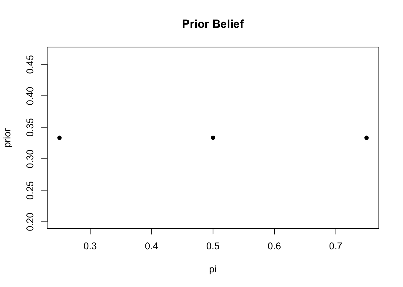
We are going to calculate with Bayes rule for each of these equations, but remember that we showed above that the denominator for all three equations are identical, and in fact are just the sum of the three numerators. Because of this, we are just going to focus on the three numerators.
So numerator one is going to be:
\[ P(\pi=.25|7in10Heads) = P(7in10Heads|\pi=.25) *P(\pi=.25) \]
What is \(P(7in10Heads|\pi=.25)\) the probability of getting 7 in 10 heads for a coin that comes up heads 25% of the time? This should be a very familiar question: it’s just the binomial.
dbinom(7,10,.25)[1] 0.003089905A very small number. It’s extremely unlikely to get this.
What’s \(P(\pi=.25)\) the probability that the coin comes up heads 25% of the time? That’s just our prior belief about the prevalence of these coins, which we set above as \(1/3\).
So to calculate this numerator:
dbinom(7,10,.25)*(1/3)[1] 0.001029968Or to calculate all three at once:
post <- dbinom(7,10,pi)*prior
plot(pi,post, pch=16, main="Posterior, Un-normalized")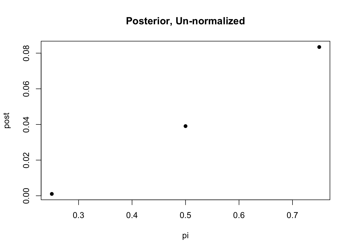
Now these numbers are not giving us real probabilities yet because we haven’t divided by the denominator \(P(Data)\), the overall probability of getting 7 in 10 heads across all three hypotheses. Remember that \(posterior \propto prior*likelihood\). Our actual posterior will be proportional to these numbers because they will all be divided by the same number. So before we even get there, we can say that the hypothesis with the highest probability is that this coin comes up heads 75% of the time.
To actually get those probabilities we divide each by the sum of the numerators:
post.norm <- post/sum(post)
plot(pi, post.norm, pch=16, main="Posterior, Normalized")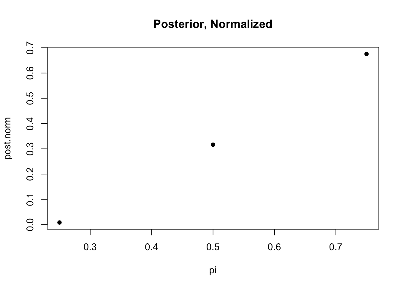
post.norm[1] 0.008338481 0.316244595 0.675416924Our posterior beliefs are that there is a less than 1% chance this coin comes up heads 25% of the time, around a 30% belief it comes up heads 50% of the time, and a 67% chance that it comes up heads 75% of the time.
It should be very clear that Bayesian analysis is sensitive to your priors. We (somewhat ridiculously) posited a prior distribution that all three coins were equally likely. But that’s not true. Unfair coins are pretty rare. So what happens if we look at the same data, and same hypotheses, but instead have a prior that there is a 95% chance this is a fair coin, with just a 2.5% chance for each of the unfair coins?
#Set priors
prior <- c(.025,.975,.025)
plot(pi, prior, pch=16, main="Prior")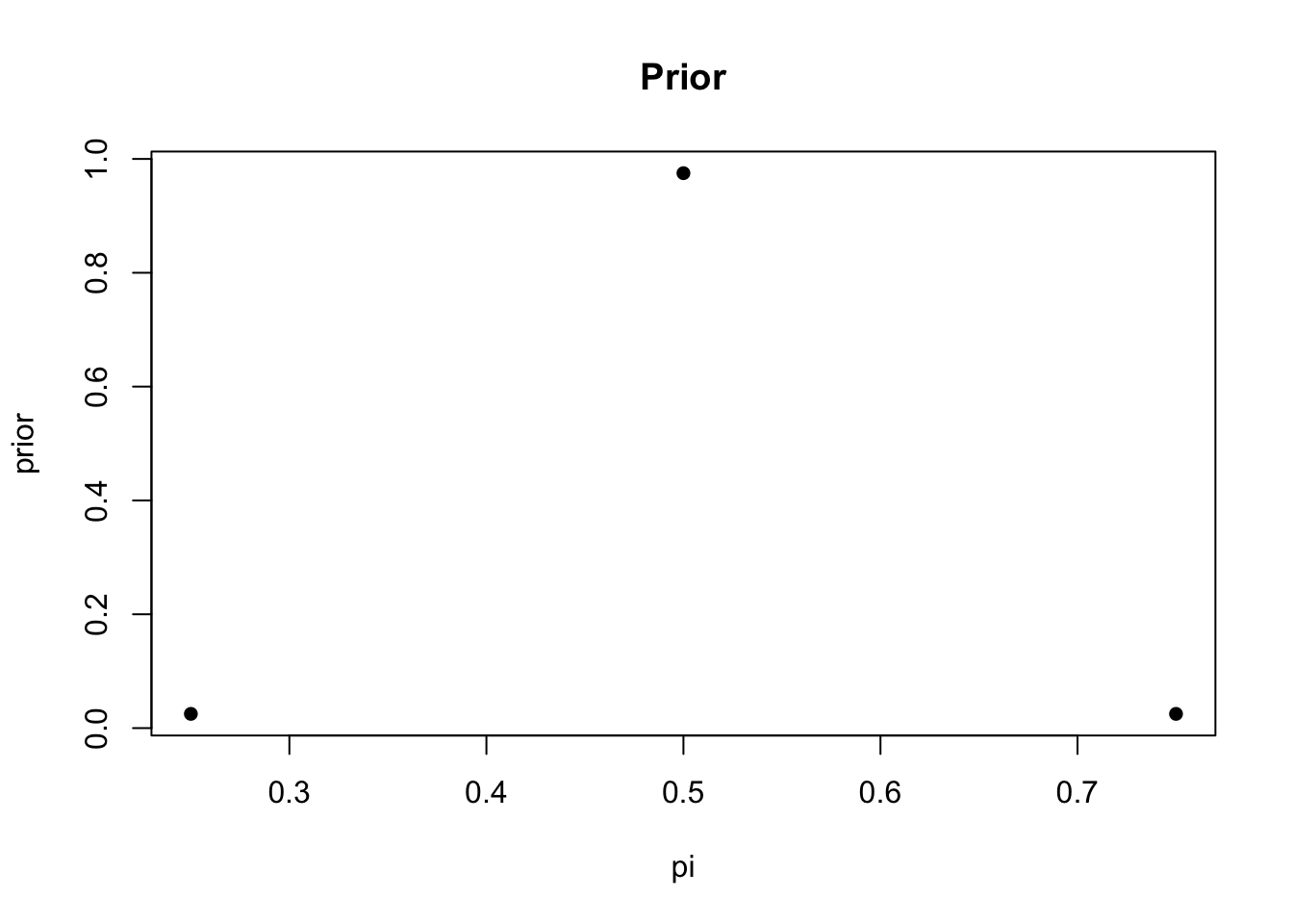
#Calculate likelihoods*priors
post <- dbinom(7,10,pi)*prior

#Normalise by dividing by the sum
post.norm <- post/sum(post)

#Display posterior
plot(pi, prior, pch=16, main="Posterior", col="gray80")
points(pi, post.norm, pch=16)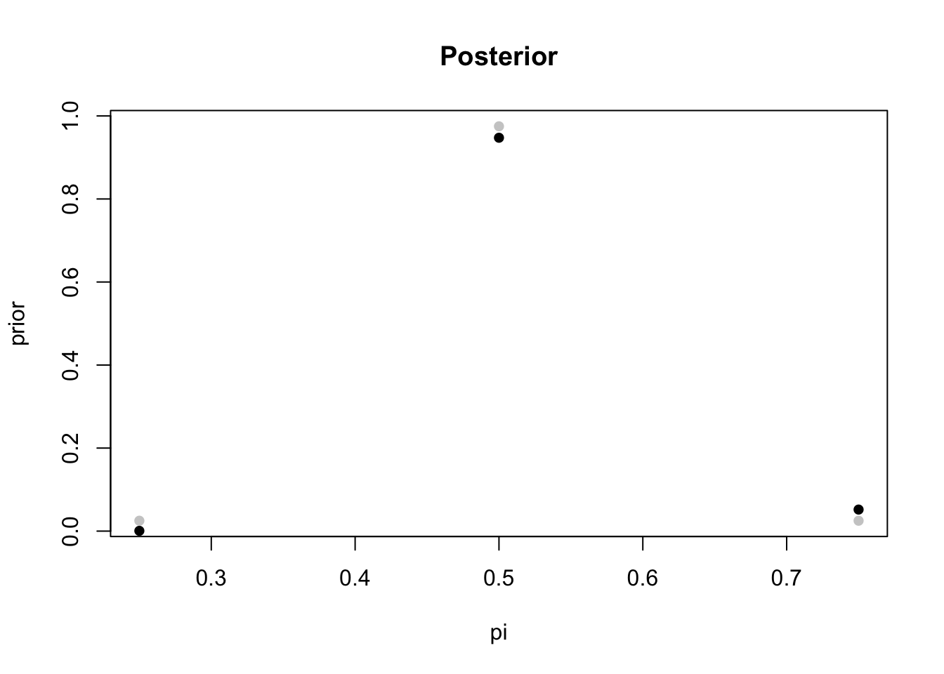
post.norm[1] 0.0006405694 0.9474733096 0.0518861210Now this data has barely moved us off our (much stronger) priors. Because we went in with the belief that unfair coins are extremely uncommon, having an observation of 7/10 heads isn’t very persuasive evidence that we are dealing with an unfair coin.
However, if we got more data that would begin to change.
What if we kept flipping and we got 70 in 100 heads?
#Calculate likelihoods*priors (This is where the change in the data is)
post <- dbinom(70,100,pi)*prior

#Normalise by dividing by the sum
post.norm <- post/sum(post)

#Display posterior
plot(pi, prior, pch=16, main="Posterior", col="gray80")
points(pi, post.norm, pch=16)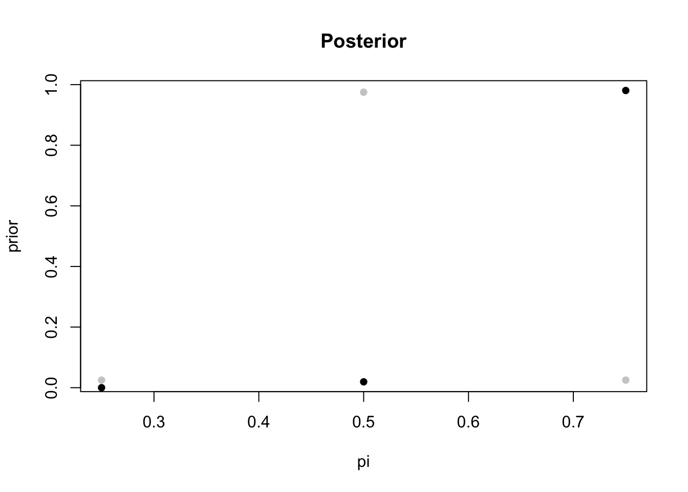
post.norm[1] 8.065957e-20 1.936790e-02 9.806321e-01That data overwhelmed our strong priors and we end up with a high degree of certainty that this is an unfair coin.
Because of the way that we set this up this is extremely easy to scale up to nearly-continuous hypotheses. What if we want to test the probability of many possible \(pi\) from 0 to 1?
pi <- seq(0,1,.001)Now we have 1001 priors from 0 to 1.
Again, let’s assign these equal probabilities, which is just 1 divided by the number of hypotheses:
prior <- rep(1/1001,1001)
plot(pi, prior, type="l", main="Prior")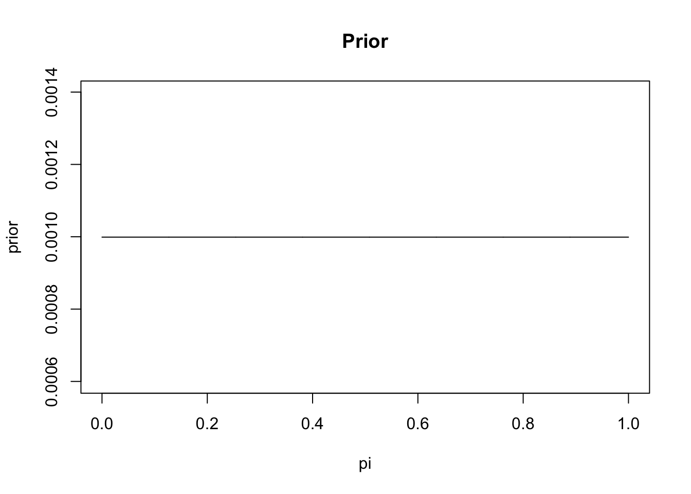
And then let’s run this through Bayes formula with the data that we have 7 heads in 10 flips:
post <- dbinom(7,10,pi)*prior
post.norm <- post/sum(post)

plot(pi, post.norm, type="l", main="Posterior")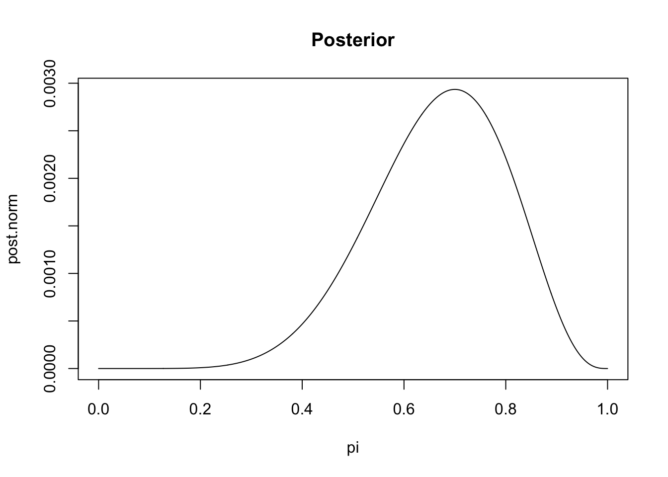
Now we have a posterior distribution across our possible hypotheses.
When we were doing frequentist statistics we could only accept or reject the null hypothesis. The nice thing here is that we now have a distribution from which we can make actual probability claims on.
So for example: given these data, what is the probability that this coin comes up heads more than 50% of the time? That’s just adding up the probability mass in the curve to the right of .5:
sum(post.norm[pi>.5])[1] 0.8860734There is an 88.6% chance that this coin comes up heads more than 50% of the time given our data.
What about a better prior that more accurately shows that unfair coins are rare. For these sort of probability questions we can use the beta distribution, which is a random variable that assigns density to values between 0 and 1. We are going to generate it and divide by the sum so that the numbers add up to 1. (Don’t worry too much about how the beta distribution works, just think about this more continuously describing the prior distribution of possibilities.)
prior <- dbeta(pi, 100,100)
prior <- prior/sum(prior)
plot(pi, prior, type="l", main="Strong Prior")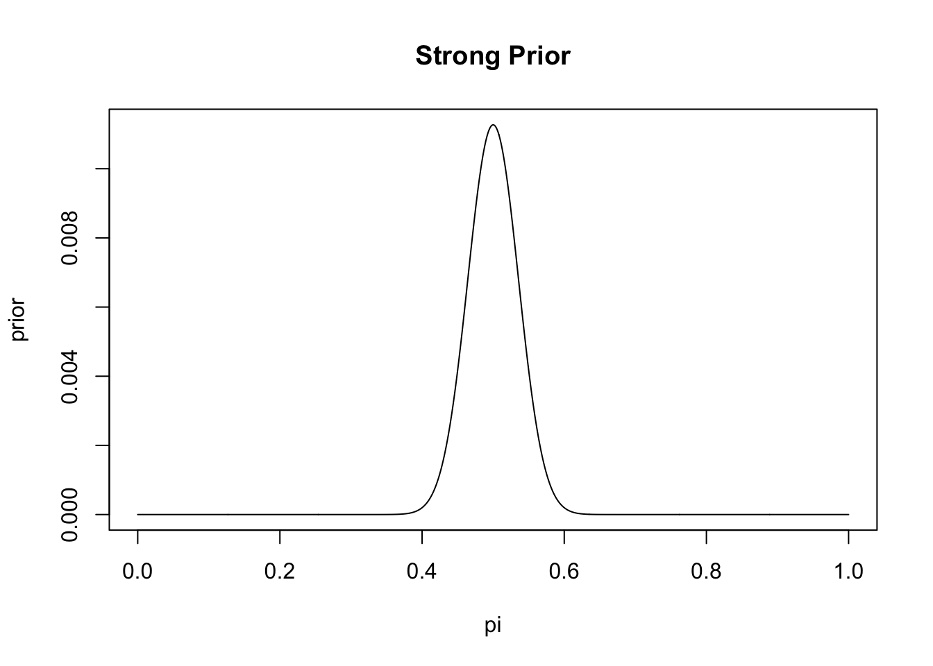
Applying Bayes rule and our observation of 7 heads in 10 flips:
post <- dbinom(7,10,pi)*prior
post.norm <- post/sum(post)
plot(pi, prior, type="l", col="gray80", main="Posterior")
points(pi, post.norm, type="l")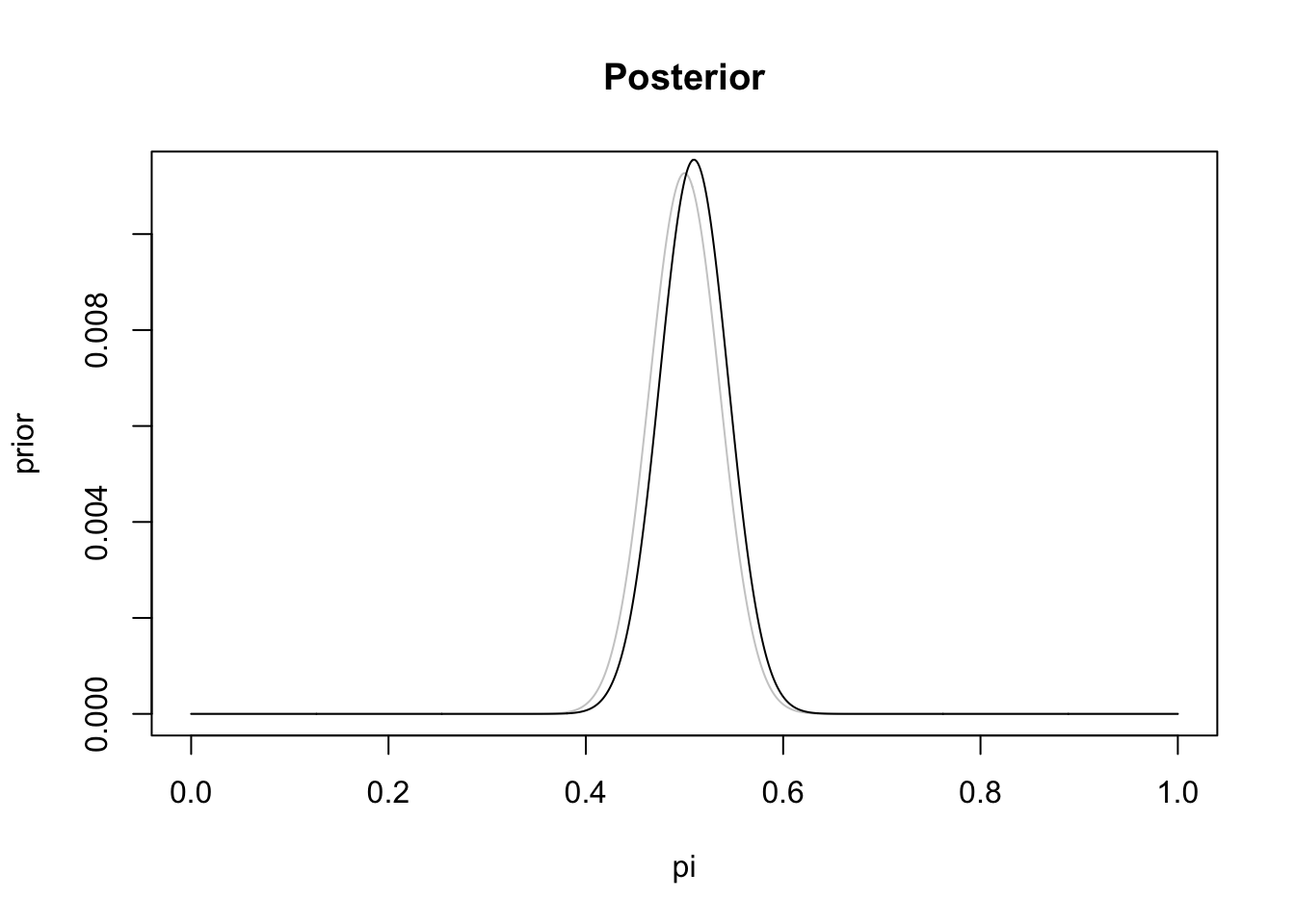
With this small amount of data our posterior distribution is barely different from our prior distribution.
But if we scale up to a world where we have 70 heads in 100 flips:
post <- dbinom(70,100,pi)*prior
post.norm <- post/sum(post)
plot(pi, prior, type="l", col="gray80", main="Posterior")
points(pi, post.norm, type="l")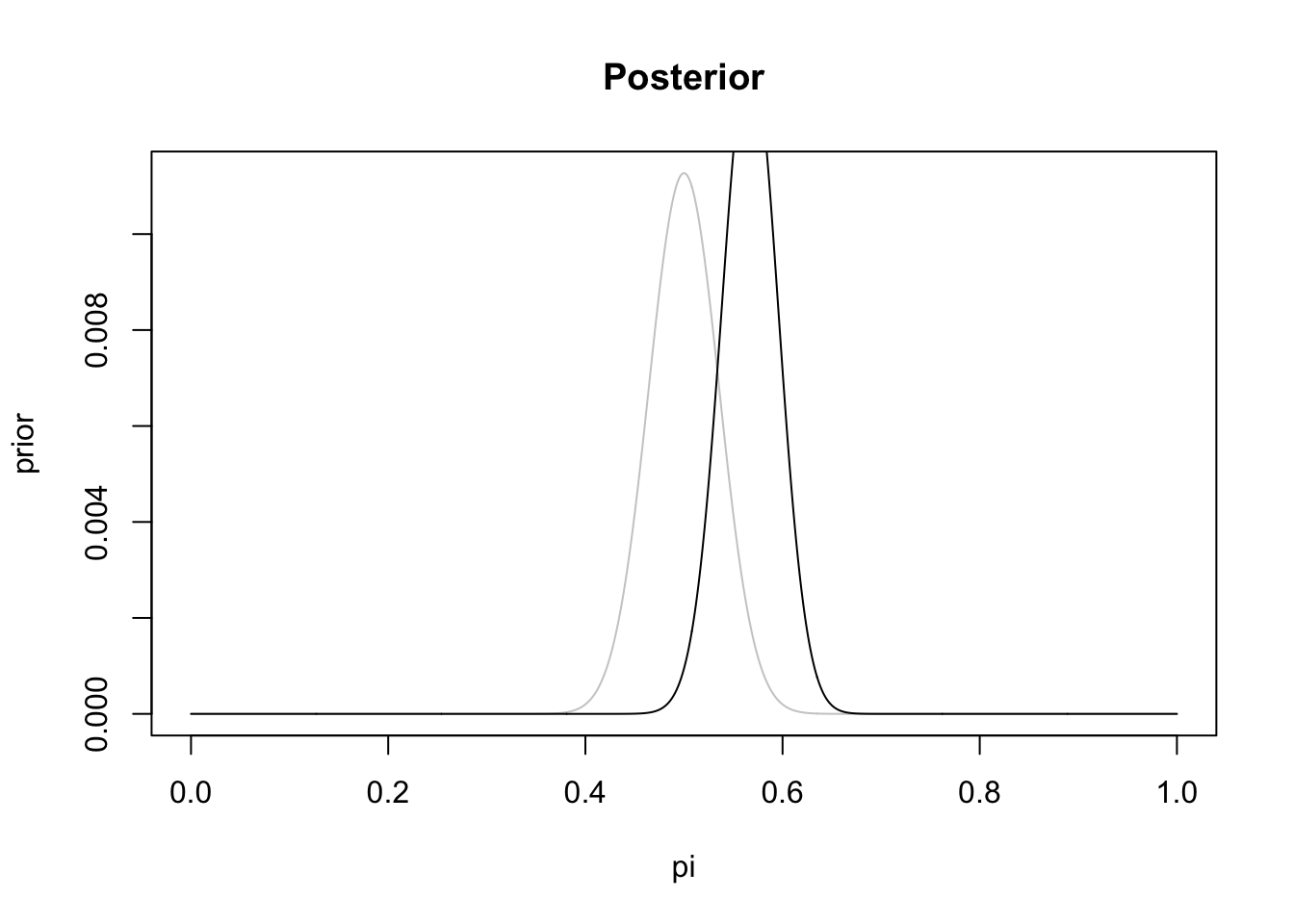
Our posterior changes more significantly.
Again, we can answer questions with the distribution that we could never with frequentist statistics. What’s the probability that this coin comes up heads between 55% and 60% of the time?
sum(post.norm[pi<.6]) - sum(post.norm[pi<.55])[1] 0.6016363About 60%.
What are the two points of this distribution where 95% of the probability mass lies?
#Calculate cumulative probability
cumu.post <- cumsum(post.norm)
#Find the boundaries
pi[min(which(cumu.post>=.975))]
[1] 0.622pi[max(which(cumu.post<=.025))][1] 0.509The 95% credible interval (the Bayesian equivalent of a confidence interval) runs from 50.9% to 62.2%.
How could we apply this to the real world?
The easiest application is to a scenario where we are interrogating a probability, because that maps cleanly on to the coin flip example that we have been working with.
Let’s say that we have the following poll of 1000 people on whether they support a Democratic (1) or Republican (0) candidate
set.seed(27)
x <- rbinom(1000,1,.52)
mean(x)
[1] 0.514where 51.4% support the Democratic candidate.
In hypothesis testing world we do a t.test with a null hypothesis that
t.test(x, mu=.50)
    One Sample t-test

data:  x
t = 0.88534, df = 999, p-value = 0.3762
alternative hypothesis: true mean is not equal to 0.5
95 percent confidence interval:
 0.4829693 0.5450307
sample estimates:
mean of x
    0.514
And we see that the probability of observing these data if the truth was that the race is tied is .376 or around 38%. As such we almost certainly would fail to reject the null hypothesis.
How would we deal with this in a Bayesian fashion?
Let’s first define a prior. Maybe this race is a toss-up, so we can center our prior on 50%, and have it cover most probabilities between 40 and 60%:
dem.support <- seq(0,1,.01)
prior <- dbeta(dem.support, 50,50)
prior <- prior/sum(prior)

plot(dem.support, prior, type="l", main="Prior")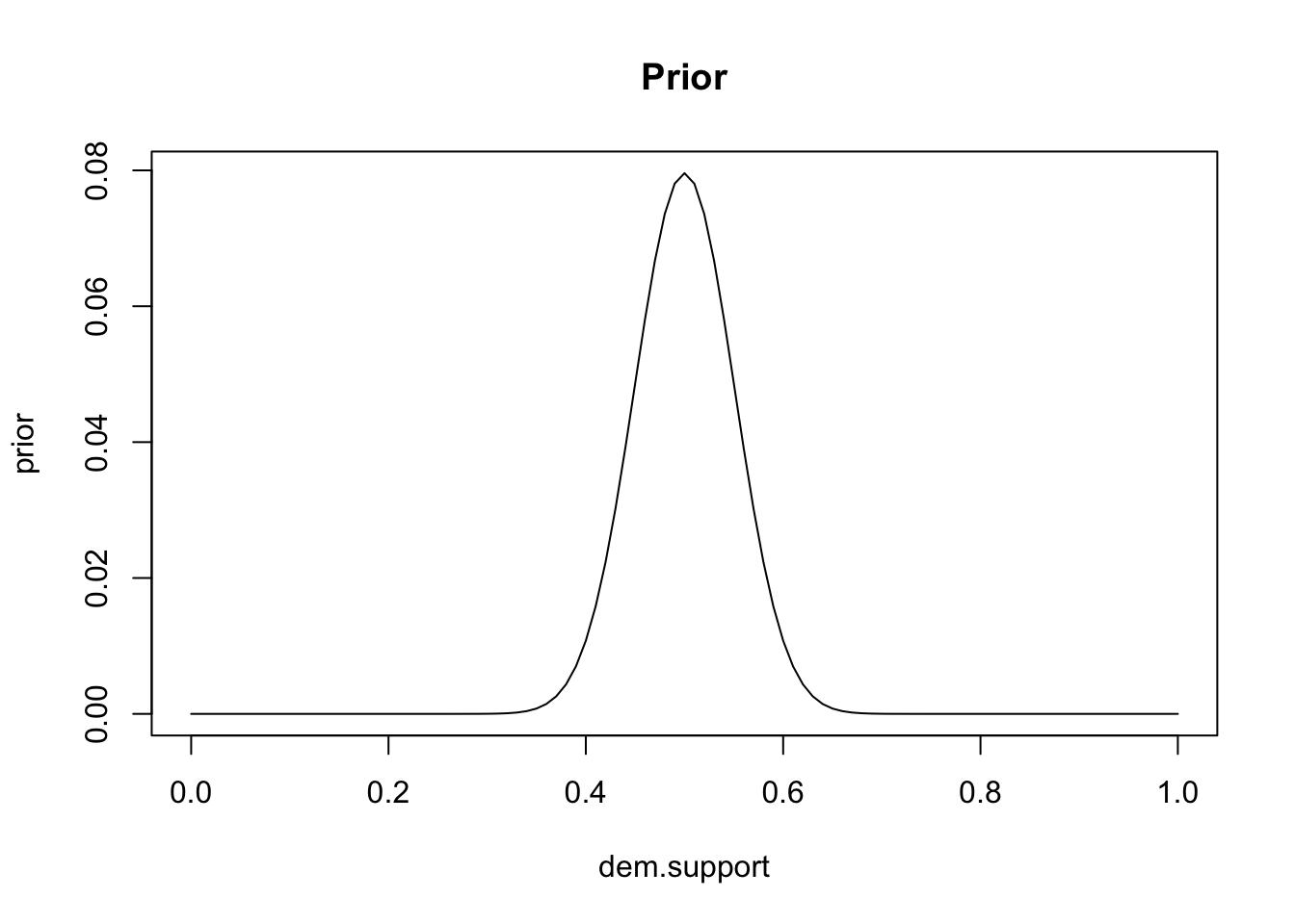
And then we consider Bayes formula for all our hypotheses: that the true dem support is 0%, 0.01%, 0.02%, filtered through our data where 514 out of 1000 people support the dem candidate:
post <- dbinom(514,1000,dem.support)*prior
post.norm <- post/sum(post)

plot(dem.support, prior, type="l", main="Prior", col="gray80")
points(dem.support, post.norm, type="l")
abline(v=.5, lty=2)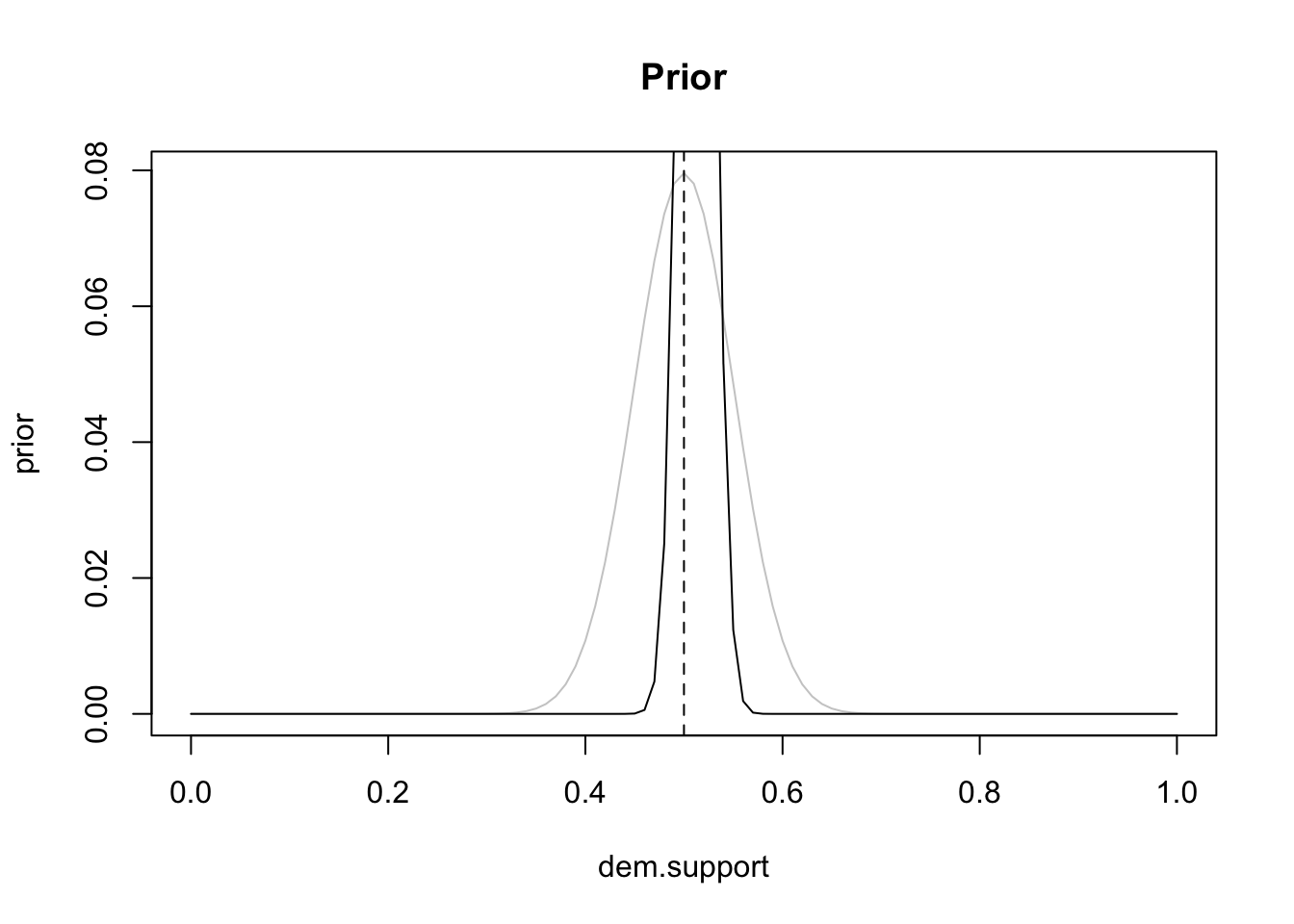
Unlike frequentist statistics where we can only say “We cannot reject the idea that the race is tied”, here we can give way more specific guidance.
What is the probability that the democratic candidate will win comfortably, with over 55% of the vote:
sum(post.norm[dem.support>=.55])[1] 0.01442396Not large. Just 1.4% probability of that occurring.
Or calculate the credible interval:
#Calculate cumulative probability
cumu.post <- cumsum(post.norm)
#Find the boundaries
dem.support[min(which(cumu.post>=.975))]
[1] 0.54dem.support[max(which(cumu.post<=.025))][1] 0.47What gets more helpful with Bayesian statistics is that we can actually have more informative priors.
What if there has already been some polling in this race: there have been three polls all with n=1000 with the results 51%, 55%, and 49.5%.
You don’t need to know this part, but we could combine these into a prior by inputting the number of successes as the first parameter and the number of failures as the second parameter:
prior <- dbeta(dem.support, 510+550+495, 490+450+505)
prior <- prior/sum(prior)
plot(dem.support, prior, type="l", main="Prior")
abline(v=.5,lty=2)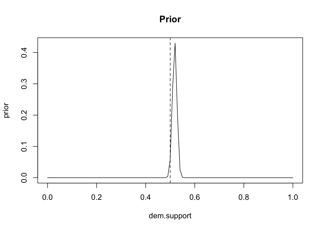
Now with this more informative prior we actually get a more certain answer from adding in our poll:
post <- dbinom(514,1000,dem.support)*prior
post.norm <- post/sum(post)
plot(dem.support, prior, type="l", main="Posterior", col="gray80")
points(dem.support, post.norm, type="l")
abline(v=.5,lty=2)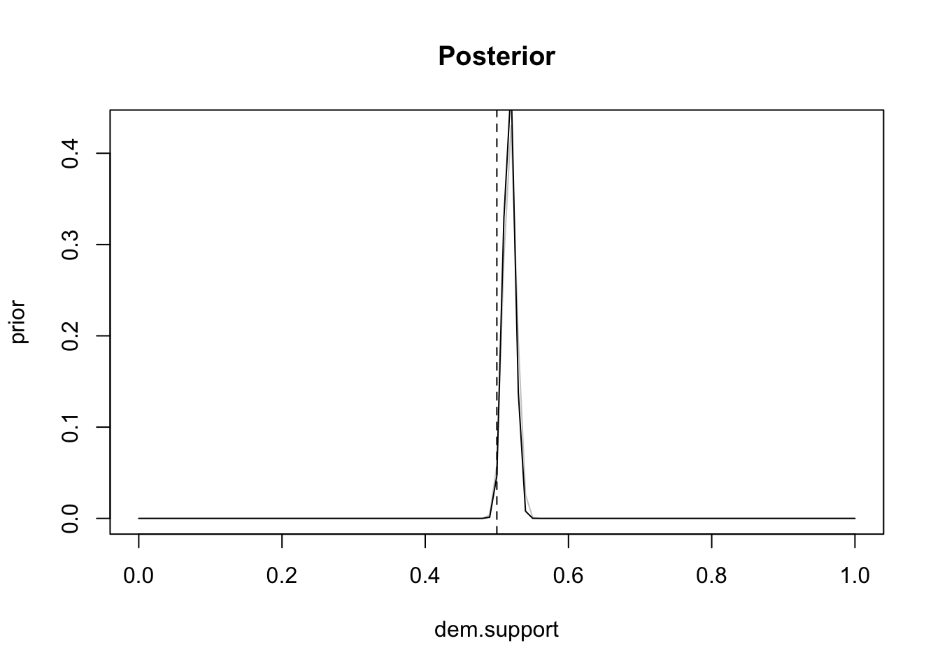
Now our credible interval is:
#Calculate cumulative probability
cumu.post <- cumsum(post.norm)
#Find the boundaries
dem.support[min(which(cumu.post>=.975))]
[1] 0.53dem.support[max(which(cumu.post<=.025))][1] 0.49Which is narrower despite having the same data!
Is this what Bayesian analysis looks like in the real world? It can! For something like a poll aggregator Bayesian analysis can look just like this.
But in reality most Bayesian analysis does not build the posterior distribution in the way that we have done here: enumerating all possible values of the posterior (the hypotheses), calculating the \(likelihood*prior\) for each, and then normalizing so that all the possibilities add up to 1.
How Bayesian analysis actually works is calculating the posterior in a slightly more complicated, but ultimately more computationally efficient, way: through sampling possible values of the posterior. I can’t walk you through how this works completely, but we can use what we have learned to build the intuition.
To start, we are going to calculate the same posterior we did above for a proportion. To be clear: this is completely unnecessary. It was not difficult for us to say: this candidate can get any proportion from 0 to 1; which one is most likely given the data and our prior? But consider us having to use Bayesian analysis for a bivariate regression where we have to estimate both an intercept and a slope. Now we would have to calculate the posterior for each combination of alphas and betas. If we have a regression with an intercept and two slopes now we have to calculate the posterior for each unique combination of all three…. you can see how this could quickly get to a level where it would be analytically intractable to actually calculate the posterior for all the possible combinations of values.
Instead of enumerating every possible value of the posterior, we are going to (intelligently) sample from it. By sample from it I mean that we are going to calculate certain values of the posterior in a systematic way that reveals where the posterior has the highest probability. Rather than sweeping through all possible values of the posterior, instead we are going to program a random walk across the values of the posterior. We are going to write this in a way that we randomly move around the values of the posterior, but in such a way that we more often visit the more likely values.
The recipe for the random walk we will use is the Metropolis algorithm. Here is what it is going to do:
In the end, the random walk should spend the most time (time being number of steps in the loops) at the values of the posterior that are most likely, and less time at values that are less likely.
Let’s build it for our poll. We are going to use the same data as above (514 of 1000 supporting the Democrat), and the same toss-up prior. First we need a function that returns the posterior height at any candidate value of \(p\). That is just likelihood times prior, the same thing we have been computing all along:
post.poll <- function(p) {
  if (p <= 0 || p >= 1) return(0)  #p has to be a probability
  dbinom(514, 1000, p) * dbeta(p, 50, 50)
}
Now we program the walk.
set.seed(19104)
#The random walk will take 20,000 steps
n.iter <- 20000
p.draws <- rep(NA, n.iter)

#We will start at 50%, but this doesn't actually matter too much
p.cur    <- 0.5                    #start somewhere
post.cur <- post.poll(p.cur)
step     <- 0.02                   #how big a step we propose

#Loop 20000 times
for (i in 1:n.iter) {
  p.prop    <- p.cur + rnorm(1, 0, step)   #propose a nearby value
  post.prop <- post.poll(p.prop) # Calculate posterior probability at new step
  #move there with probability equal to the ratio of the two heights
  if (runif(1) < post.prop / post.cur) {
    p.cur    <- p.prop
    post.cur <- post.prop
  }
  p.draws[i] <- p.cur                       #write down where we are
}

#throw away the early "burn-in" steps that depend on where we started
p.draws <- p.draws[2001:n.iter]
We now have 18,000 sampled values of \(p\) that should be weighted towards where the posterior is highest.
We can easily look at where the walk took us over its run. Here is the first 100:
plot(1:100, p.draws[1:100], type="l")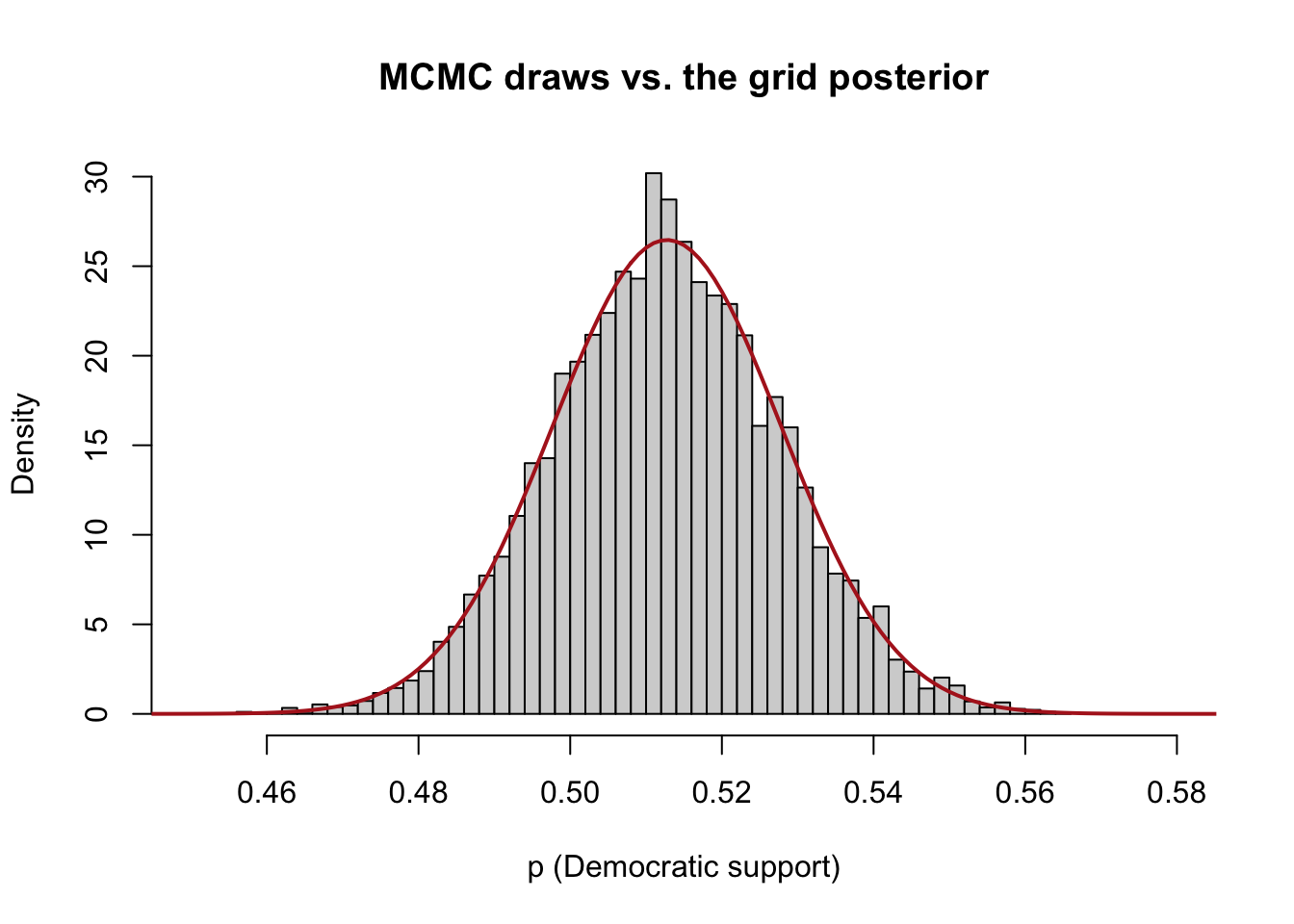
It shifted around over the course of the 100, spending a bit more time where the posterior probability is highest.
And here are all 18,000:
plot(1:length(p.draws), p.draws, type="l")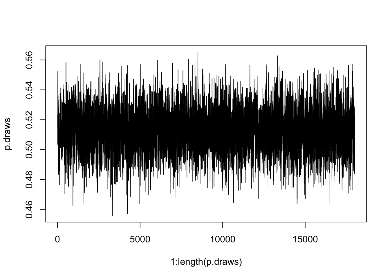
That’s not that helpful to look at, but note that it never strayed far from this interval. By seeing that the posterior probability got really small as it got away from here, it didn’t have to go down to 10% or up to 90% to calculate the probability.
So does this walk actually reproduce the posterior? Let’s put a histogram of the sampled values against the fully manually calculated posterior:
#Fine-grid posterior as the benchmark
p.grid <- seq(0, 1, 0.001)
prior  <- dbeta(p.grid, 50, 50); prior <- prior / sum(prior)
grid.post <- dbinom(514, 1000, p.grid) * prior
grid.post <- grid.post / sum(grid.post)

hist(p.draws, breaks = 40, freq = FALSE, xlim = c(.45, .58),
     main = "MCMC draws vs. the grid posterior",
     xlab = "p (Democratic support)")
#overlay the grid posterior (rescaled to a density for comparison)
points(p.grid, grid.post / mean(diff(p.grid)), type = "l", col = "firebrick", lwd = 2)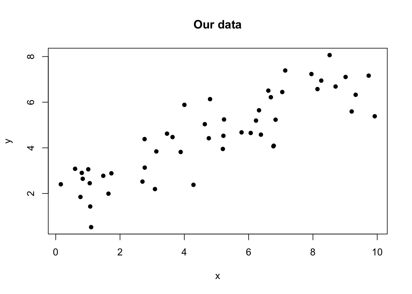
The histogram of sampled values traces out the same curve the grid gave us. Again: we didn’t get this by calculating every possible value, but instead semi-randomly wandering around the posterior space, recording where we spent more time because the probability was higher.
To answer any question we summarize our vector of posterior values, very similar to the way that we summarize bootstrap resamples:
mean(p.draws) #posterior mean[1] 0.5126977quantile(p.draws, c(.025, .975)) #95% credible interval 2.5% 97.5%
0.4836261 0.5422909 mean(p.draws > 0.5) #P(Democrat ahead)[1] 0.8002778A posterior mean of about 0.513, a credible interval of roughly 0.48 to 0.54, and about an 80% probability the Democrat is ahead. These are the same numbers the grid gave us, because the two methods compute the same thing through different methods.
But for a single parameter this really was pointless: the grid was easier and gave an identical answer. The reason it matters is when we scale up the number of hypotheses dramatically.
Everything we did above had a single parameter for which we wanted a posterior. But again: when we move into regression models every unique combination has a possible posterior probability, and checking all of them becomes incredibly inefficient.
Let’s do the same sampling technique for a regression.
We are going to do the exact same thing: posit a possibility, calculate the posterior probability, and let the walker shift around finding which possibilities have the highest probabilities. The only difference is that a possibility is now a pair of numbers instead of one, so the walker roams a two-dimensional plane of candidate \((\alpha, \beta)\) pairs instead of a one-dimensional line of candidate \(p\) values.
Let’s make dead-simple data where we know the answer, an intercept of 2 and a slope of 0.5:
set.seed(19104)
n <- 50
x <- runif(n, 0, 10)
y <- 2 + 0.5 * x + rnorm(n, mean = 0, sd = 1)
plot(x, y, pch = 16, main = "Our data")
We need to generate the posterior probability for any possible combination of values. Now, the calculation of \(likelihood*prior\) is slightly more complicated in this case, but works on the same principle. I’m not going to fully explain the below code, and I don’t expect you to understand it. It is enough to know that what this is doing is \(likelihood*prior\)
#Log-score of a candidate line: bigger (less negative) = better fit
log.post <- function(alpha, beta) {
  sum(dnorm(y, mean = alpha + beta * x, sd = 1, log = TRUE)) +
  dnorm(alpha, 0, 10, log = TRUE) + dnorm(beta, 0, 10, log = TRUE)
}
Now we turn the walker loose. It is the identical sampler from the poll, with one change: each step proposes a small move in the intercept and the slope at the same time, so it wanders the two-dimensional plane instead of the line.
set.seed(19104)
#Number of steps
n.iter <- 20000
draws <- matrix(NA, nrow = n.iter, ncol = 2)
colnames(draws) <- c("alpha", "beta")

#Starting point
alpha.cur <- 0; beta.cur <- 0
#Posterior for starting point
lp.cur <- log.post(alpha.cur, beta.cur)
step <- 0.15

for (i in 1:n.iter) {
  #Move alpha a small amount
  alpha.prop <- alpha.cur + rnorm(1, 0, step)
  #Move beta a small amount
  beta.prop  <- beta.cur  + rnorm(1, 0, step)
  #Calculate posterior of proposed step
  lp.prop    <- log.post(alpha.prop, beta.prop)
  #move with probability equal to the ratio of the two heights
  if (runif(1) < exp(lp.prop - lp.cur)) {
    alpha.cur <- alpha.prop; beta.cur <- beta.prop; lp.cur <- lp.prop
  }
  draws[i, ] <- c(alpha.cur, beta.cur)
}
draws <- draws[2001:n.iter, ]
Here is where the walker spent its time, plotted in the plane of intercept-slope pairs:
plot(draws[, "alpha"], draws[, "beta"], pch = 16, cex = .3,
     col = rgb(0, 0, 0, .1),
     xlab = "Intercept (alpha)", ylab = "Slope (beta)",
     main = "Where the walker went")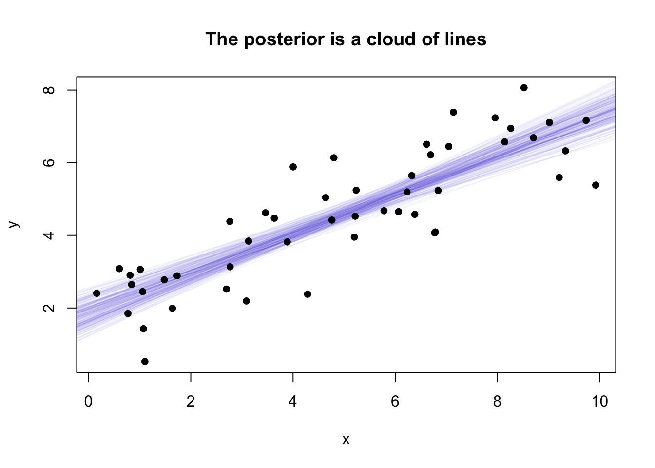
That cloud is the posterior over \((\alpha, \beta)\). It leans on a diagonal because a steeper slope has to be paired with a lower intercept to keep the line running through the data, so the two are not independent.
What did we actually sample? On the poll each draw was a single number and the whole thing was a vector. Here each draw is a pair, an intercept and a slope, which is to say each draw is a whole line. So the posterior is a distribution over lines. We can see that literally by drawing a few hundred of the sampled lines faintly over the data:
plot(x, y, pch = 16, main = "The posterior is a cloud of lines")
for (i in seq(1, nrow(draws), length.out = 200)) {
  abline(a = draws[i, "alpha"], b = draws[i, "beta"], col = rgb(.2, .2, .8, .05))
}
points(x, y, pch = 16)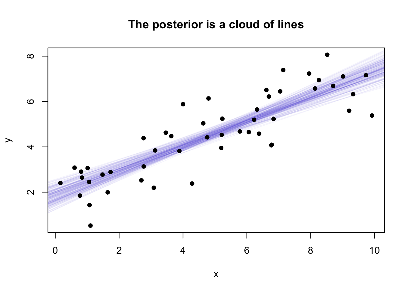
Where the lines bunch tightly the posterior is confident; where they fan out it is uncertain. That fan is the Bayesian answer to “what is the relationship between x and y”: not one best line, but the full set of lines the data find plausible.
We can also pull the two columns apart and look at each on its own. The intercept draws are the posterior for \(\alpha\), the slope draws are the posterior for \(\beta\), and each is just a distribution we can histogram exactly like any coin or poll posterior we built earlier:
par(mfrow = c(1, 2))
hist(draws[, "alpha"], breaks = 40, main = "Posterior: intercept", xlab = "alpha")
hist(draws[, "beta"],  breaks = 40, main = "Posterior: slope",     xlab = "beta")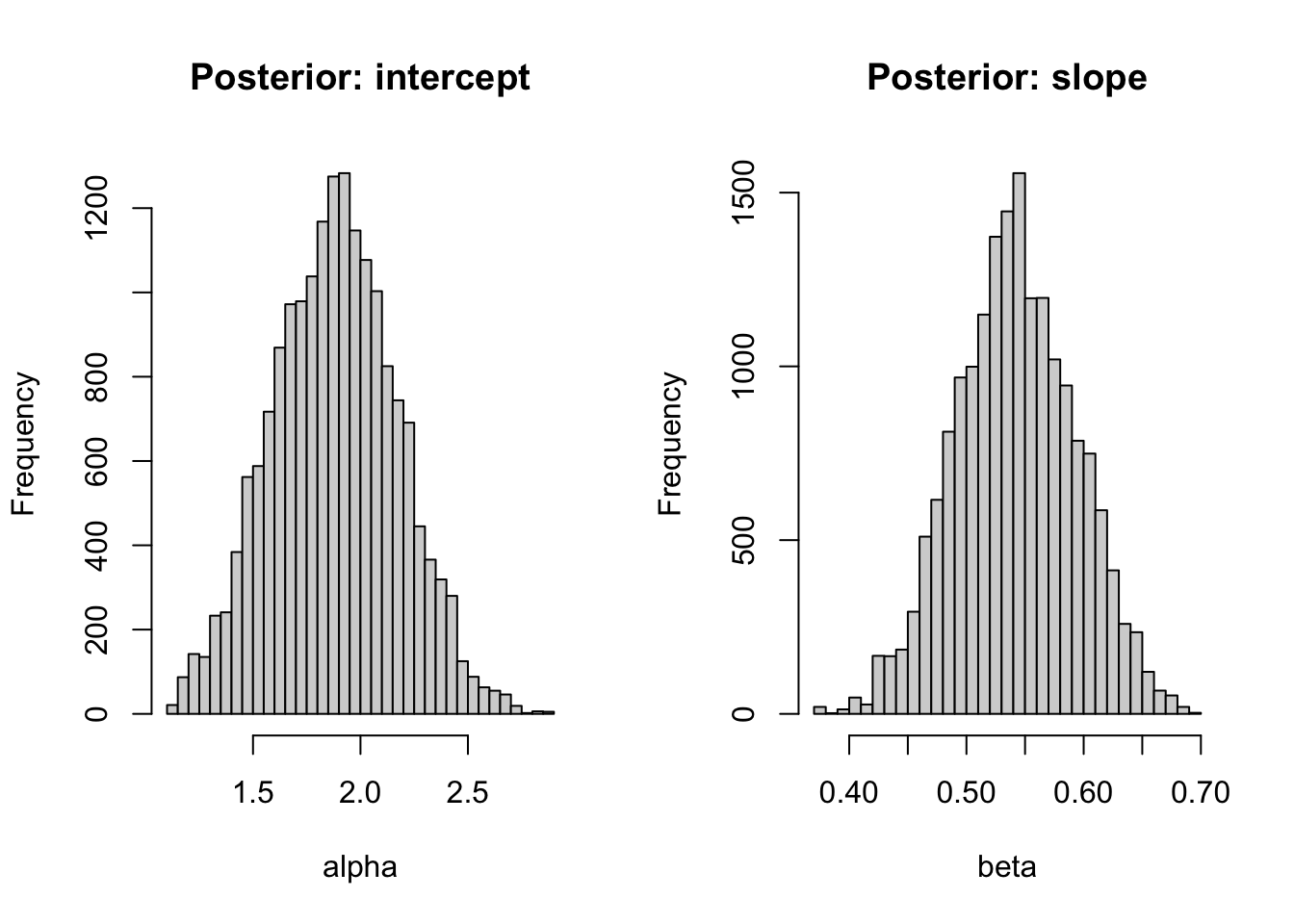
par(mfrow = c(1, 1))From here it is all summarizing those columns of draws, the same as always:
colMeans(draws) #posterior means alpha beta
1.8811654 0.5418772 quantile(draws[, "beta"], c(.025, .975)) #95% credible interval for the slope 2.5% 97.5%
0.4414345 0.6426614 mean(draws[, "beta"] > 0) #P(slope is positive)[1] 1The slope posterior is centered near 0.54, with a credible interval of about 0.44 to 0.64 and essentially a 100% probability the slope is positive.
Least squares gives the same interval:
confint(lm(y ~ x)) 2.5 % 97.5 %
(Intercept) 1.3682705 2.432993
x 0.4453066 0.634123Going from one parameter to two did not substantially change what it is that we were doing. We could scale this up substantially (say a regression with 10 predictors) and all we would change is that each step would propose a random step across many dimensions. We would still just have to compare two values (the posterior at where we are and where we propose going).
This is the whole reason we sample instead of enumerate. Manually checking all values explodes as you add parameters: a hundred candidate values per unknown is ten thousand points in two dimensions, a hundred trillion in seven, and hopeless past that. The random walk gets around this by never trying to determine the whole posterior, instead smartly going where the probability is highest.
That’s all that “real” Bayesian software does. When people fit Bayesian models in practice they use tools like Stan, brms, or PyMC.
At this point you might be asking: if Bayesian statistics gives more intuitive answers, why did we spend an entire semester doing frequentist statistics?
A few reasons:
The social sciences overwhelmingly use frequentist methods. If you read a paper in political science, economics, or sociology, you will see p-values and confidence intervals. You need to understand these tools to read the literature.
Bayesian computation used to be extremely difficult. It is only in the last 20-30 years that computers have become fast enough to do serious Bayesian analysis routinely. The frequentist framework was developed in part because the math was tractable with pencil and paper.
The prior is genuinely controversial. Two researchers with different priors can reach different conclusions from the same data. In some fields, this is seen as unacceptable. In others, it is embraced.
With enough data, the two approaches agree. For most of the problems we have tackled this semester – with hundreds or thousands of observations – the frequentist and Bayesian answers are nearly identical. The differences matter most with small samples or strong prior information.
You should probably understand both frameworks, and there are some interesting things you can do with Bayesian analysis with big data. But if you are only going to know one thing, it’s the frequentist framework.
The frequentist framework gives you a rigorous, prior-free methodology for evaluating evidence. The Bayesian framework gives you a principled way to incorporate prior knowledge and make direct probability statements. Best to think of them as complements.