eval <- seq(-5,60,.001)
plot(eval,dchisq(eval,10,ncp=12), type="l", main="Population",
     xlab="Values",ylab="Density", ylim=c(0,0.06), xlim=c(0,65))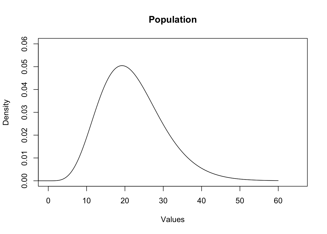
📄 Download the R code from this chapter
📝 Download the class handout for this chapter
In the previous chapter we learned key lessons about sampling variability and how it relates to our ability to infer things about an unknown population. Specifically, we learned about the Central Limit Theorem, which tells us that our sample mean is drawn from a sampling distribution of sample means that has a known shape.
In this chapter we are going to extend this knowledge to think through how to practically make use of this information when we don’t know what the shape of the population is.
First, to review, in the process of making inferences there are three distributions of data that we care about. It is imperative that you understand the differences between these three things.
First is the population that we are sampling from. This can look like anything: it can be normal, it can be binomial, it can be uniform, it can be a random variable that we don’t have a name for. Anything. To show this, let’s consider this Chi-squared distribution to be the population. Like the Uniform and Normal we covered in ContinuousRVs, it’s just another continuous random variable with its own PDF; here the point isn’t the details of the distribution, it’s that we can sample from an arbitrary shape and the CLT will kick in regardless. You don’t have to know anything about the Chi-squared distribution, other than the fact that it doesn’t look like a normal distribution. So here is our population:
eval <- seq(-5,60,.001)
plot(eval,dchisq(eval,10,ncp=12), type="l", main="Population",
xlab="Values",ylab="Density", ylim=c(0,0.06), xlim=c(0,65))
This is what is generating the values when we take a sample. We are unlikely to get anything less than (say) 5. We are most likely to get values around 20. We are unlikely to get values greater than 50. This is a non-symmetrical distribution so we aren’t likely to have a sample where the mean and median are equal. Again, we can think of this as the population or the “data generating process”.
Alright, now we will take a sample of 50 from this population:
set.seed(19104)
x <- rchisq(50,10,ncp=12)
head(x)
[1] 17.17206 15.50880 29.22219 18.31710 31.47061 20.98213What does that sample look like?
plot(density(x), main="Sample", xlab="Value", ylim=c(0,0.06), xlim=c(0,65))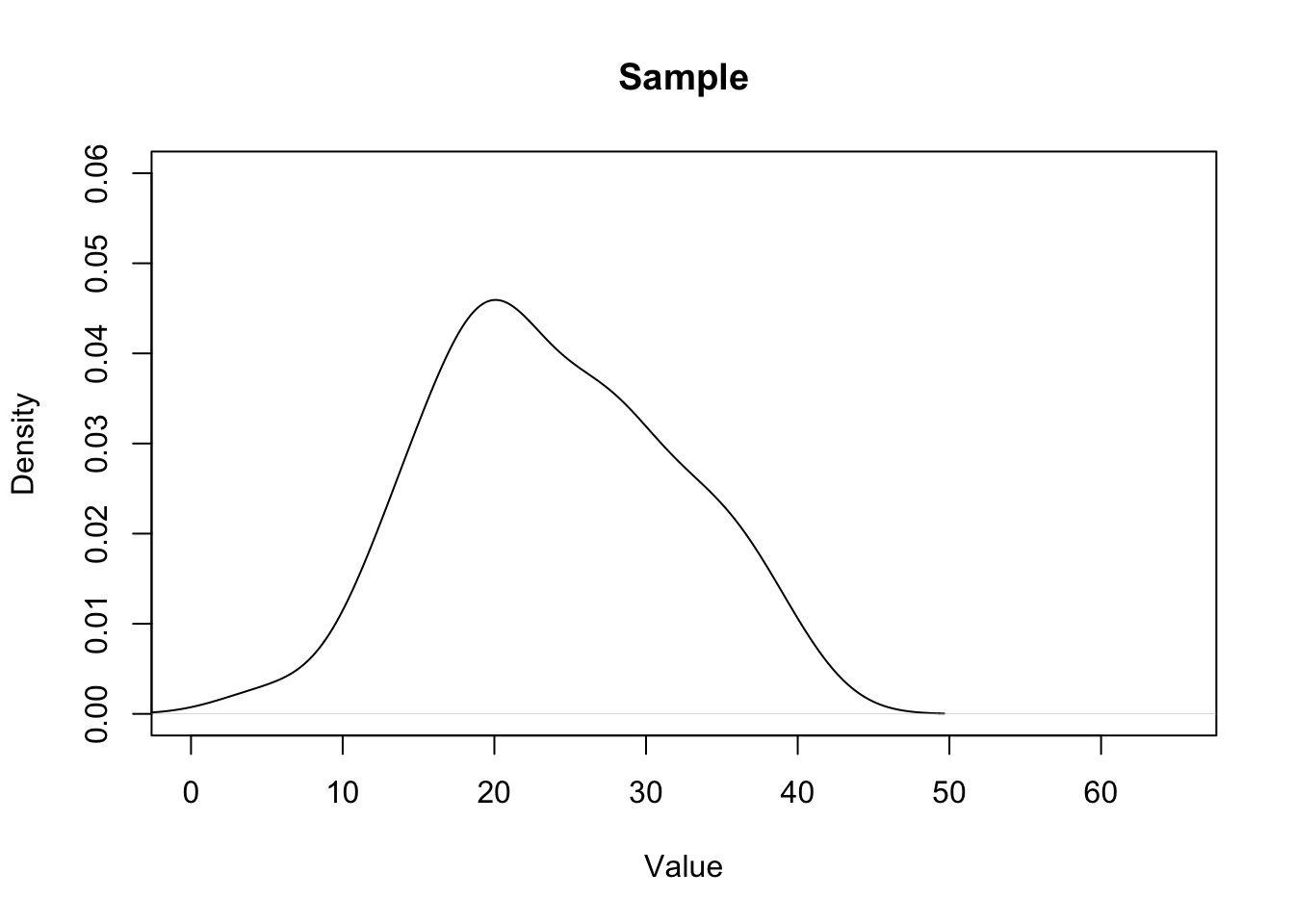
We can think of each sample as being a rough approximation of the population it was generated from. The larger the sample size, the more the sample will look like the population. (However, critically, this is NOT what the Central Limit Theorem is.)
Let’s plot the population beside the density of our sample to see how close of approximation we got:
plot(density(x), main="Sample", xlab="Value", ylim=c(0,0.06), xlim=c(0,65))
points(eval,dchisq(eval,10,ncp=12),col="firebrick", type="l")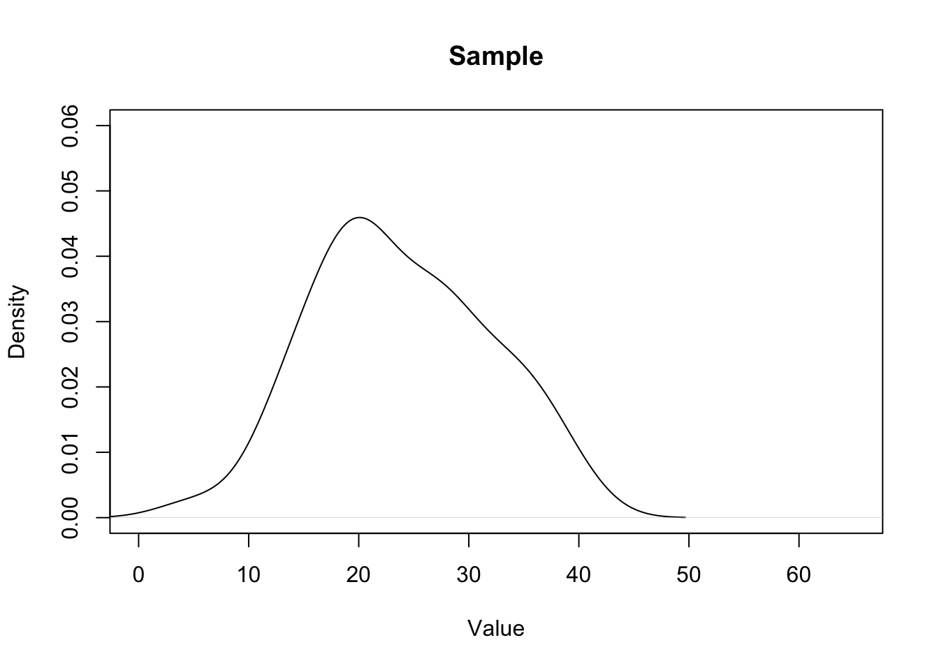
It’s definitely…. in the ballpark?
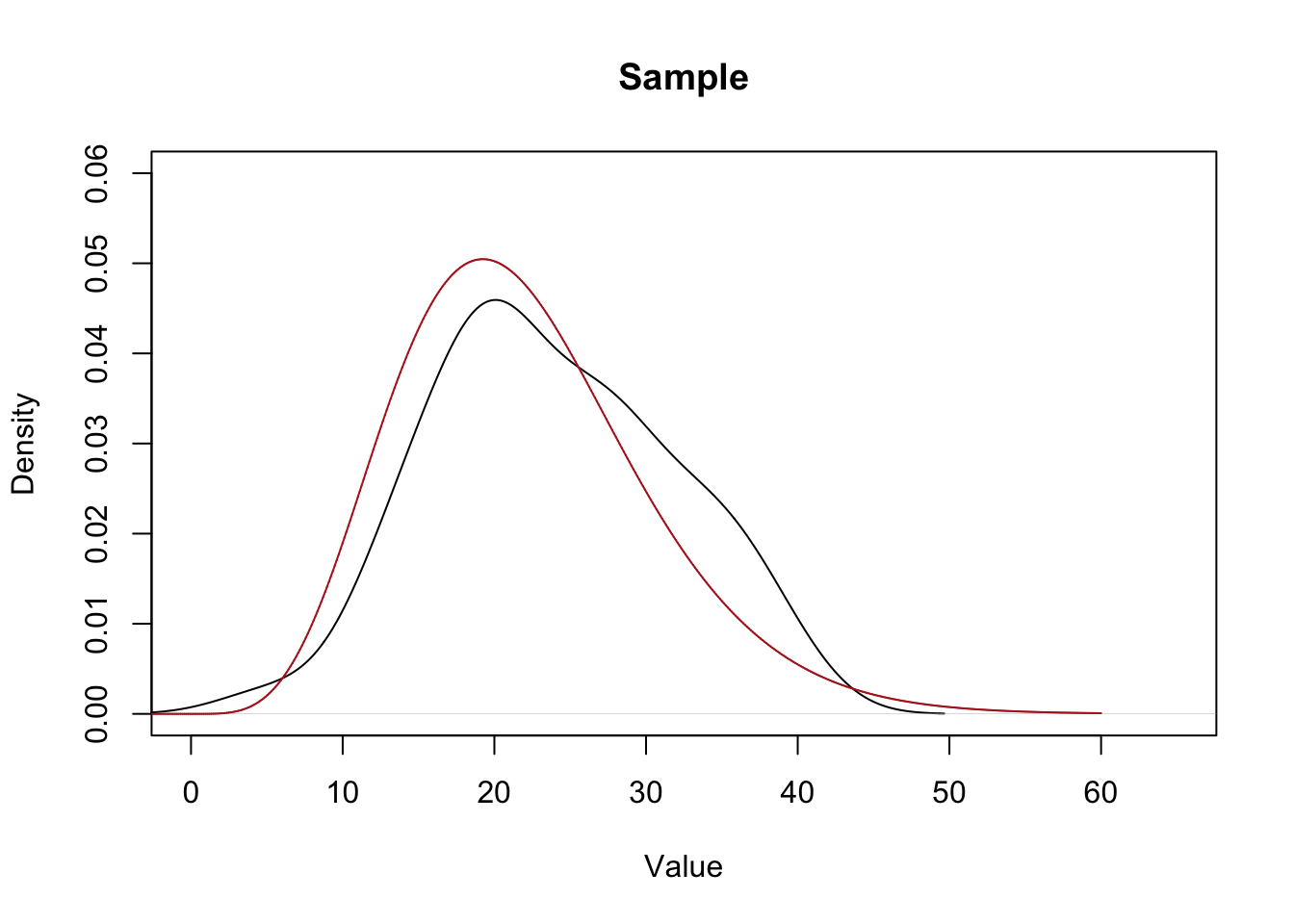
Every time we take a sample we will get a distribution of data that will be a rough approximation of the population. Here’s 9 more samples:
par(mfrow=c(3,3))
for(i in 1:9){
samp <- rchisq(50,10,ncp=12)
plot(density(samp), main="Sample", xlab="Value", ylim=c(0,0.06), xlim=c(0,65))
points(eval,dchisq(eval,10,ncp=12),col="firebrick", type="l")
}
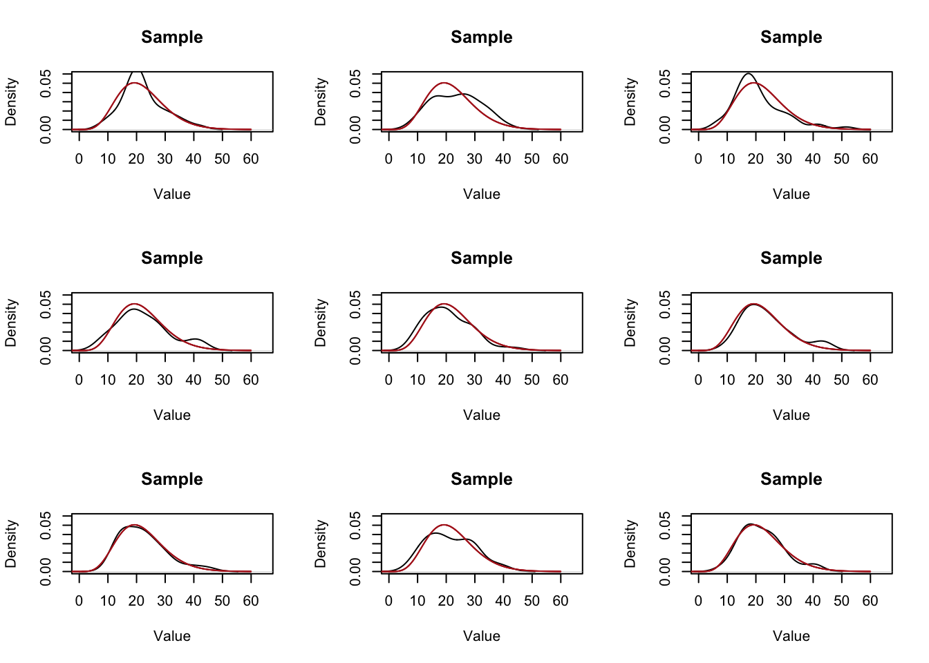
So all of these “roughly” approximate the population….. but how good a job do they do? We can eyeball it but that’s not a great answer…. We intuitively also know that if we up the sample size we will do a “better” job of estimating the distribution in the population:
par(mfrow=c(3,3))
for(i in 1:9){
samp <- rchisq(1000,10,ncp=12)
plot(density(samp), main="Sample", xlab="Value", ylim=c(0,0.06), xlim=c(0,65))
points(eval,dchisq(eval,10,ncp=12),col="firebrick", type="l")
}
But again, we can’t put numbers onto this.
The key thing we have learned is that, while it’s ultimately futile to ask “How much will my sample look like the population for a sample size of \(n\)?”, we can predict how much the sample mean will look like the true population expected value.
To reiterate this: statistics does not have a good way of estimating how close the distribution of the sample will be to the distribution of the population. We know that as the sample size increases they will look increasingly the same, but “how much will the distribution of my sample deviate from the distribution of the population for an \(n\) of 50” is not an answerable question.
But! We know that the sample mean is itself a random variable, and that random variable has a distribution defined by :
\[ \bar{X_n} \sim N(\mu=E[X], \sigma^2 = V[X]/n) \]
So, we can’t answer “how much deviation is there in the distribution of our sample compared to the population for an n of 50?”, but we can answer: “how much deviation in the sample mean will there be for an n of 50”.
Specifically, each sample mean for an n of 50 will be drawn from this normal distribution, based on my knowledge that the \(E[X]=22\) and \(V[X]=68\).
mean.eval <- seq(15,29,.001)
plot(mean.eval, dnorm(mean.eval, mean=22, sd=sqrt(68/50)), type="l",
     main="Sampling Distribution of the Sample Mean",
     xlab="Value of Sample Mean",
     ylab="Density")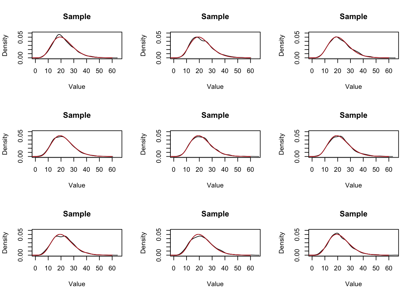
We can prove this to ourselves by repeatedly sampling and taking a bunch of sample means and plotting their density compared to this sampling distribution.
sample.means <- rep(NA, 10000)

for(i in 1:10000){
  sample.means[i] <- mean(rchisq(50,10,ncp=12))
}

plot(mean.eval, dnorm(mean.eval, mean=22, sd=sqrt(68/50)), type="l",
     main="Sampling Distribution of the Sample Mean",
     xlab="Value of Sample Mean",
     ylab="Density")
points(density(sample.means), type="l", col="darkblue")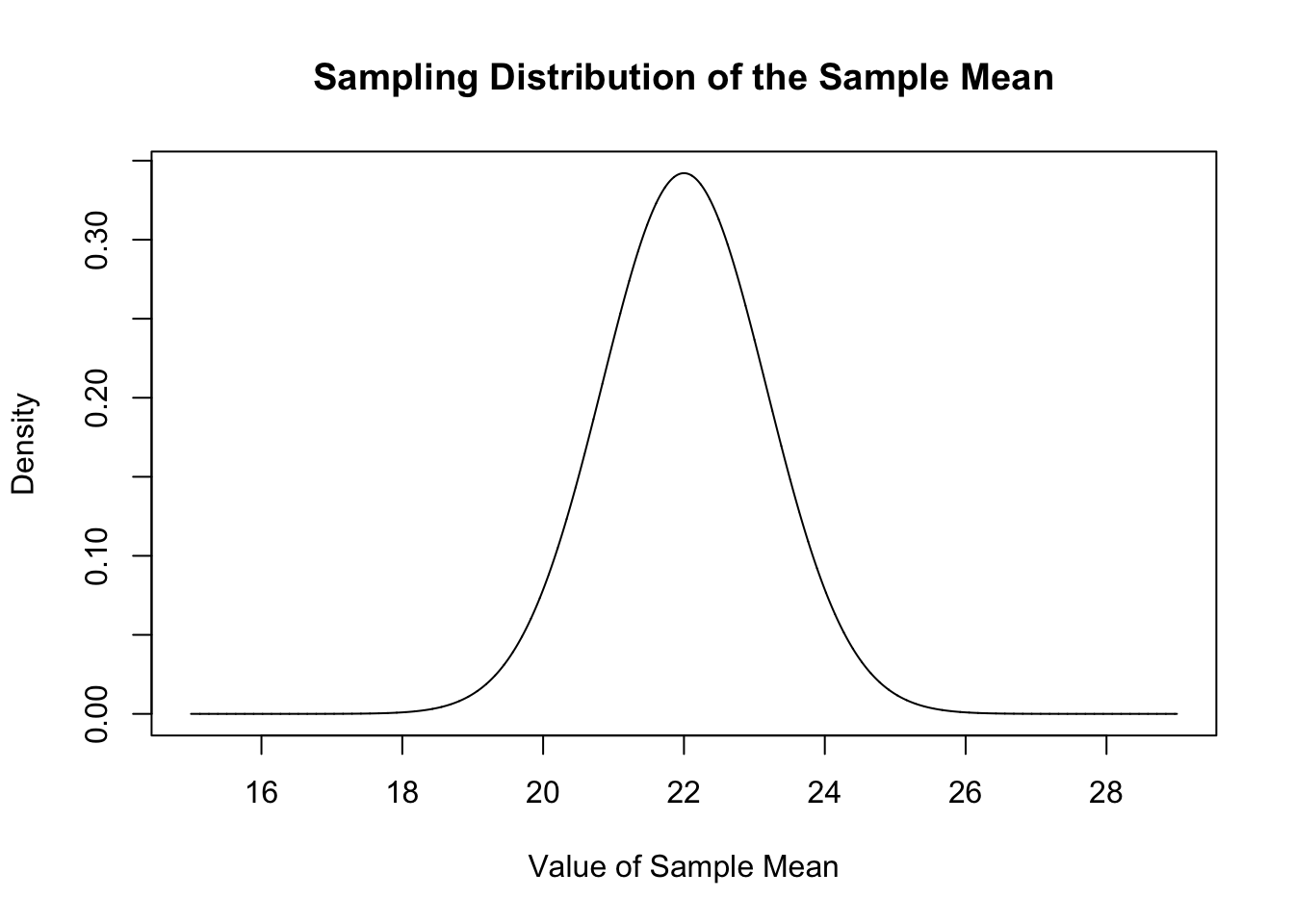
They are the same distribution.
This is the third distribution we care about: the sampling distribution of an estimate that we form using our sample. Here we are looking at the sampling distribution of the sample mean, but many estimates and accompanying sampling distributions are possible.
While we cannot determine “how much will the distribution of our sample vary from the population distribution?” we can determine, “how much will the sample mean vary from sample to sample?”
Because the random variable that generates sample means is known, we can ask: what proportion of sample means will be within 2 of the true population mean. In other words, what is the probability mass that is between the two lines below:
source("https://raw.githubusercontent.com/marctrussler/IIS-Data/main/NormalShader.R")

plot(mean.eval, dnorm(mean.eval, mean=22, sd=sqrt(68/50)), type="l",
     main="Sampling Distribution of the Sample Mean",
     xlab="Value of Sample Mean",
     ylab="Density")
normal.shader(16,28,22,sqrt(68/50),value.one = 20, value.two = 24, between=T)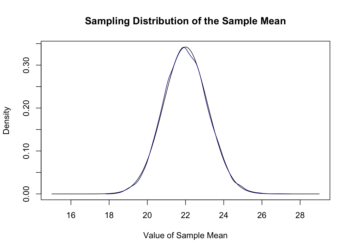
Because we know exactly what shape that sampling distribution is, we can answer this question precisely using the normal distribution:
pnorm(24,22,sqrt(68/50)) - pnorm(20,22,sqrt(68/50))[1] 0.9136522There is a 91% chance a sample mean drawn from this distribution will be between 20 and 24.
Is that true? We already drew a bunch of random samples and took the sample means from this Chi-Squared population, so is it true that 91% of them are in between those two bounds?
mean(sample.means>=20 & sample.means<=24)[1] 0.9194Yes!
What is the range in which 70% of all estimates will lie?
Well that’s leaving 15% in the left tail so:
qnorm(.15, 22, sqrt(68/50))[1] 20.79132#How much above and below the mean
val <- 22 - qnorm(.15, 22, sqrt(68/50))
22 + val[1] 23.2086822 - val[1] 20.79132That range contains 70% of all estimates.
Is that true?
mean(sample.means>=20.79 & sample.means<=23.21)[1] 0.7035Yes!
How can we think about the relationships between these three distributions: the population, sample, and the sampling distribution of the mean?
The sampling distribution of the sample mean is related to the sample because each sample produces a sample mean. The sampling distribution of the sample mean is intricately related to the population, because the shape of the normal distribution is driven by the expected value and variance of the population.
The population and sample are clearly related. The distribution of the sample is generated by the population so it is a rough (but not perfect) approximation. We have seen that the mean of a sample is equal to the expected value of the population, in expectation (the law of large numbers). However it is also true that the variance of a sample is a rough approximation of the population level variance:
sample.vars <- rep(NA, 10000)

for(i in 1:10000){
  sample.vars[i] <- var(rchisq(50,10,ncp=12))
}
summary(sample.vars)
Min. 1st Qu. Median Mean 3rd Qu. Max.
24.91 57.05 66.47 68.03 77.44 145.34 Indeed, this fact, that the variance of the sample is a good approximation for the variance of the population, is what we are going to exploit next to move our whole operation forward.
So far we have seen that we can predict what the distribution of sample means will look like if we know the expected value and variance of the population we are pulling from… But the whole point is that we don’t know the population!
Consider, again, running a poll of \(n=500\) to understand the distribution of income in a certain population. If we did that we would get the following information:
median(x)[1] 69627.39mean(x)[1] 73117.75sd(x)[1] 20454.85var(x)[1] 418400760The median income in our sample of 500 is around 69k and the mean is 73k. The standard deviation of our sample is around 20k.
We do not know anything about the population it came from. (I mean, if you go look at the code you can see exactly where I generated this data from, but let’s keep up the charade and say that we don’t know.)
In the examples above we were able to say: ok here is what the population is like, and therefore I can derive exactly what the sampling distribution of the sample mean would look like. Here we also want to generate a sampling distribution, but how are we going to do that when we don’t know anything about the population?
To draw a sampling distribution we need a \(\mu\) and a \(\sigma\) (the two ingredients for any normal distribution).
As the first step, I’m going to change the question from “What does the population distribution of income look like?” to a much easier question to answer: What if the expected value in the population is $70,000 (approximately the median income in the US)?
That immediately helps us because we can now say: if the expected value in the population is 70000, then the sampling distribution of the sample mean will be centered on that value. We don’t need to worry about where the true expected value of the population is, because now we are explicitly positing that it is centered on 70k and seeing what falls out from that.
OK, but here’s the harder part: we need a \(\sigma\). Up to this point we have said that the sampling distribution of the sample mean is \(\sim N(\mu=E[X], \sigma^2 = V[X]/n)\). But we don’t have the variance of the population level random variable!
What can we use instead?
Well we really only have one option. We saw above that the distribution of our sample is a rough approximation of the distribution of the population, so what happens if we use the variance of our sample as a stand-in for the variance of the population?
Note that there is one additional complication to subbing in the sample variance. See below on how we actually have to start using the \(t\) distribution when we do this.
To be clear, the variance of the population is a fixed known thing. Because we are “god” here and know the truth I know that the variance of the population is around 400 million. What is the variance of our actual sample?
var(x)[1] 418400760It’s close! What would the two sampling distributions look like, once with the true variance, once with the sample variance:
eval <- seq(65000,75000,100)
plot(eval, dnorm(eval, mean=70000, sd=sqrt(4e+08/500)), type="l", col="firebrick")
points(eval, dnorm(eval, mean=70000, sd=sqrt(var(x)/500)), type="l", col="darkblue")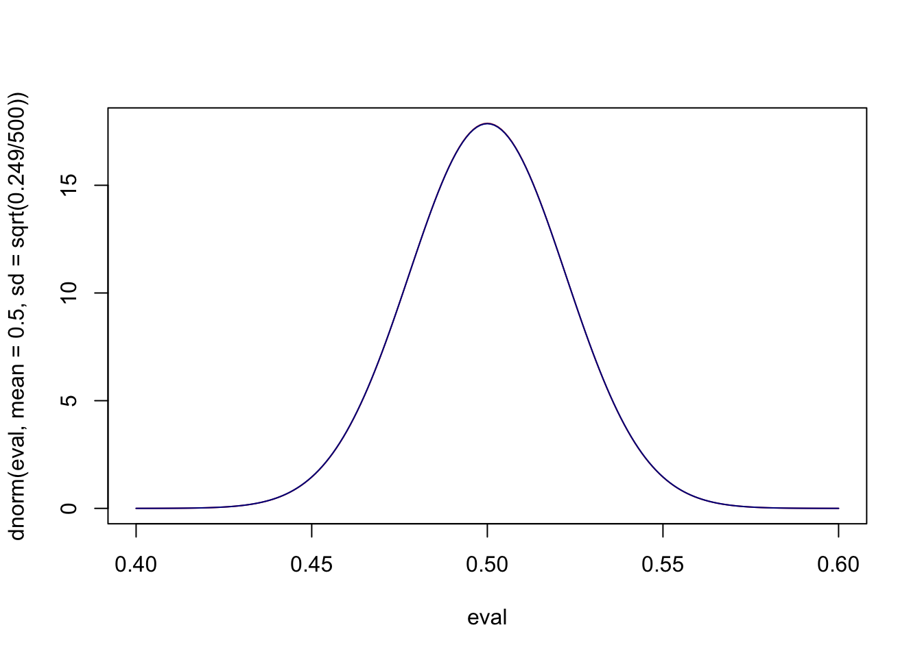
Effectively the same.
Subbing that in, we can now say: well if the truth was that the expected value of income in this population was 70k, then the sampling distribution would look like this:
plot(eval, dnorm(eval, mean=70000, sd=sqrt(var(x)/500)), type="l", col="darkblue", ylab = "Density",
     xlab="Income")
abline(v=mean(x), lty=2, lwd=2, col="firebrick")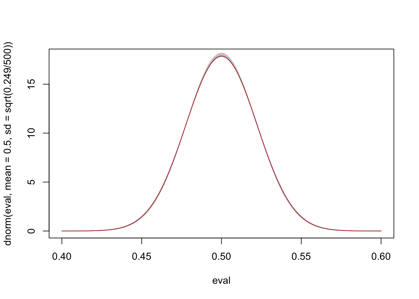
The sample mean we got (shown by the red line) is pretty extreme, relative to this distribution. As such, we may want to reject the notion that the true mean in this population is 70k.
Maybe we just got lucky this time that the sampling variance was a good stand in for the population variance. Let’s take a bunch of samples, calculate the variance of each, and plot the sampling distribution generated from each of them on top of each other to see generally how well we do:
plot(eval, dnorm(eval, mean=70000, sd=sqrt(4e+08/500)), type="l", col="firebrick")

for(i in 1:1000){
  samp.var <- var( rsnorm(500, mean = 73000, sd = 20000, xi = 2.2))
  points(eval, dnorm(eval, mean=70000, sd=sqrt(samp.var/500)), type="l", col="gray80")
}
points(eval, dnorm(eval, mean=70000, sd=sqrt(4e+08/500)), type="l", col="firebrick")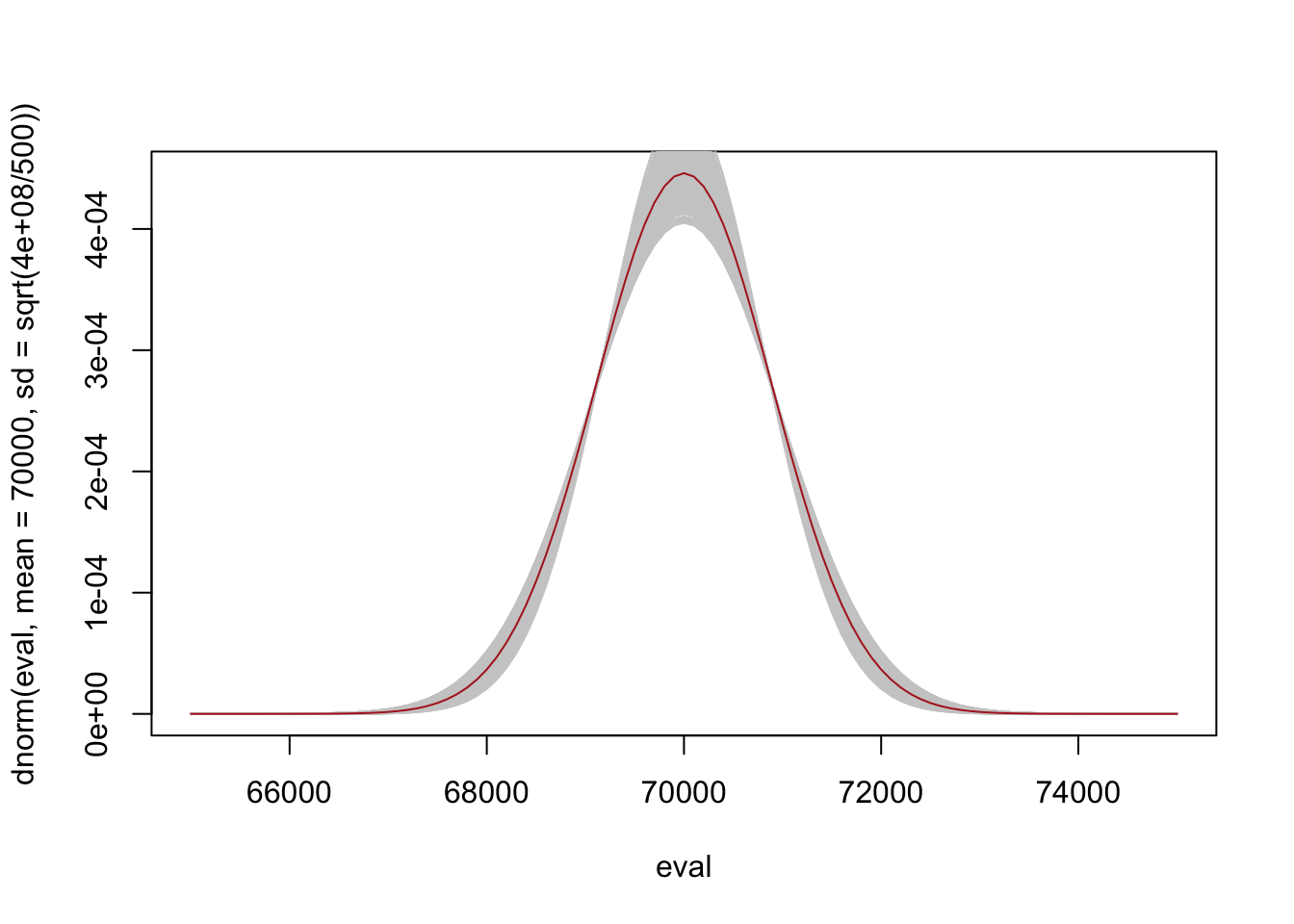
That looks pretty good! Again, here we are comparing the “true” sampling distribution that is generated using the population level variance to many sampling distributions that are generating from subbing in the sample variance to represent the population variance.
One thing to note is that the equation to calculate the sample variance (which we denote as \(S^2\)) is:
\[ S^2 = \frac{1}{n-1}*\sum_{i=1}^{n}(X_i- \bar{X_n})^2 \]
This is, effectively, the average deviation from the average. However, instead of dividing by \(n\) we divide by \(n-1\).
Why? Because. That’s why! But for real if we went through and did the math then:
\[ E\left[\frac{1}{n-1}*\sum_{i=1}^{n}(X_i- \bar{X_n})^2\right] = \sigma^2 \]
And:
\[ E\left[\frac{1}{n}*\sum_{i=1}^{n}(X_i- \bar{X_n})^2\right] \neq \sigma^2 \]
Helpfully, the var() and sd() commands automatically makes this adjustment.
So in the “real” world all we do to figure out a sampling distribution for the sample mean is to sub in the sample variance for the population variance. (With one additional complication, that we will get to).
Let’s consider what sort of question we might want to answer in the world where we don’t know the population.
Let’s take a sample mean of a small sample from the normal distribution (100 people) and look at the mean and variance:
set.seed(19104)
x <- rnorm(100,64,3)
mean(x)
[1] 63.92013var(x)[1] 7.876416Now again, In this case we know that the truth is 64, but in the real world we would not.
What we want to effectively know is where the true value might plausibly lie in relation to this value.
Is it plausible that the truth is 70? or 50? Could the truth be 0?
There are (roughly) two ways to answer this question: confidence intervals and hypothesis tests. We will cover CIs today and spend next week covering hypothesis tests.
A confidence interval is a zone that we are some percent certain contains the true population parameter. So if a 70% confidence interval ranged from \([5,10]\) that would mean that we are 70% confident the population parameter is within those bounds1.
Here is how confidence intervals work:
We think that our sample mean is drawn from a sampling distribution. We do not know what the center of that sampling distribution is (the true population mean), but we do think we can do a reasonable job of estimating the shape of the sampling distribution by using the sample variance as a stand in for the population variance.
For a confidence interval we center this sampling distribution on our sample mean. We then determine the zone where 70% (or 90%, or 95%… whatever confidence level we want) of the probability mass lies. This zone has a 70% (or 90% or 95% ) probability of containing the true population mean.
How do we put a such a confidence interval around our sample above?
We define a confidence level as \((1-\alpha)*100\), such that a 70% confidence interval implies an \(\alpha\) of .3.
For a given \(\alpha\) a confidence interval around any given sample mean is:
\[CI(\alpha) = [\bar{X_n}-z_{\alpha/2}*SE,\bar{X_n}+z_{\alpha/2}*SE]\]
Where \(z\) is the standard normal distribution.
This is just restating what I said above mathematically: to form a confidence interval we have to evaluate the standard normal distribution at \(-\alpha/2\) and \(\alpha/2\). We can take those two values and multiply them by the standard error. (Recall from Sampling that the standard error is the standard deviation of the sampling distribution, \(sd(X)/\sqrt{n}\). Here we’re using the sample-based version, \(s/\sqrt{n}\), because in the real world we don’t have \(sd(X)\).) The resulting amount above and below the sample mean will be a zone that contains the true population parameter \((1-\alpha)*100\) percent of the time.
So using that logic, the confidence interval for our sample which had a \(\bar{X_n}=63.92\) and \(s^2=7.88\) would be:
\[ \begin{aligned} se &= \sqrt{7.88/100} = .28\\ \alpha &= .3 \end{aligned} \]
#Evaluate standard normal for alpha/2
qnorm(.3/2)
[1] -1.036433\[ \begin{aligned} z_{\alpha/2}&=1.04\\ CI(\alpha) &= [\bar{X_n}-z_{\alpha/2}*SE,\bar{X_n}+z_{\alpha/2}*SE]\\ CI(\alpha) &= [63.92-1.04*.28,63.92+1.04*.28]\\ CI(\alpha) &= [63.62,64.21] \end{aligned} \]
There is a 70% chance that the true population parameter is contained within that interval.
Visually, we can think about the sampling distribution being normally distributed with a standard error of .28. We center that normal distribution on our sample mean of 63.92 and think about the area that symmetrically contains 70% of the probability mass. We think that there is a 70% chance the true population mean is in that area.
x <- seq(63,65,.001)
plot(x, dnorm(x, mean=63.92, sd=.28), type="l")
normal.shader(63,65,mu  = 63.92, sd = .28,63.62, 64.21, between=T)
abline(v=63.92)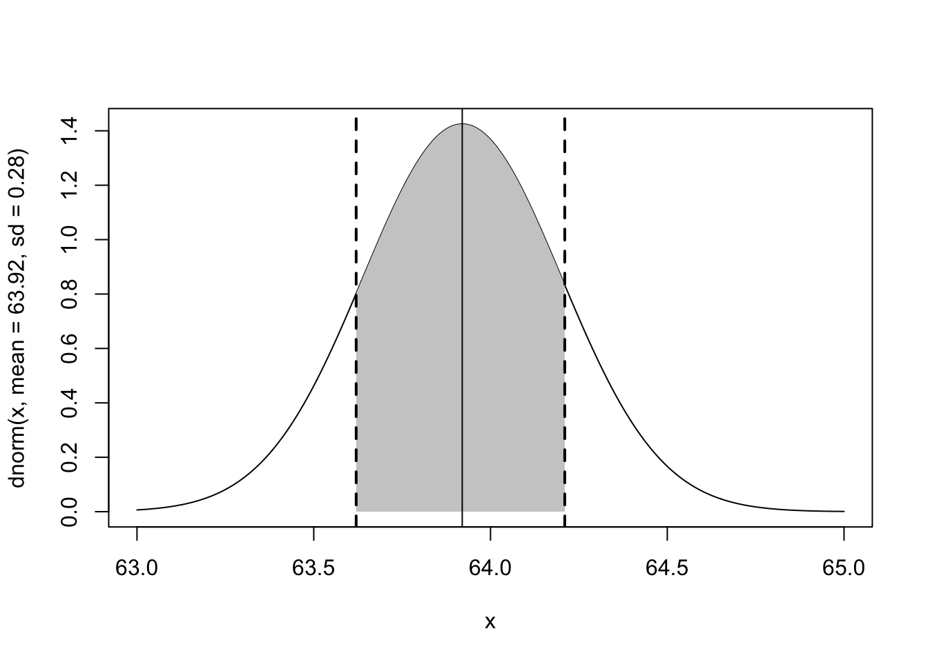
OK: so let’s prove that this is true. Let’s repeatedly sample from the same population, and using information wholly contained within that sample let’s calculate the confidence interval and test to see whether it contains the true population parameter. First let’s visualize doing this 10 times:
lower <- rep(NA,10)
upper <- rep(NA,10)

for(i in 1:10){
samp <- rnorm(100,64,3)
xbar <- mean(samp)
s2 <- var(samp)
se <- sqrt(s2/100)
lower[i] <- xbar - 1.04*se
upper[i] <- xbar + 1.04*se
}

plot( seq(63.2,65,.2),seq(1,10), type="n", xlim=c(63,65))
abline(v=64, lty=2, col="firebrick")
segments(lower, 1:10, upper, 1:10)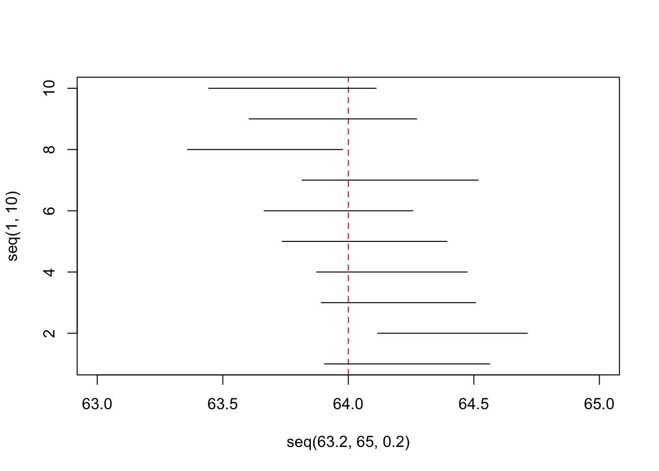
Our expectation is that 7 out of these 10 confidence intervals will contain the true population paramater. In reality 8 out of the 10 do, which is very close. To see if this is true though we can repeat this process 10,000 times:
ci.contains <- rep(NA,10000)

for(i in 1:10000){
samp <- rnorm(100,64,3)
xbar <- mean(samp)
s2 <- var(samp)
se <- sqrt(s2/100)
lower <- xbar - 1.04*se
upper<- xbar + 1.04*se
ci.contains[i] <- lower<=64 & upper>=64
}
mean(ci.contains)
[1] 0.6976Yes! 70% of similarly constructed confidence intervals contain the true population parameter.
A note on language here. Technically speaking the definition that I’ve given you: “a confidence interval has a X% probability of containing the true population parameter” is incorrect. Any given confidence interval is a real zone with 2 fixed numbers. The population parameter is also a fixed, real number. So a confidence interval either does, or does not, contain the true population parameter. There is nothing about chance to it, and some people will absolutely jump down your throat if you claim that there is a 70% chance this confidence interval contains the truth. The correct thing to say is “70% of similarly constructed confidence intervals contain the true population parameter” which jeeeeeeeeeesus this is why people hate statistics.
I’m not a professional statistician and to me it makes sense that if 70% of confidence intervals contain the truth, the probability that the one that I have contains the truth is 70%. That is technically wrong but it makes intuitive sense and I’m fine with it.
Looking at the equation for the confidence interval we can think through what makes wider or narrower confidence intervals:
\[CI(\alpha) = [\bar{X_n}-z_{\alpha/2}*SE,\bar{X_n}+z_{\alpha/2}*SE]\]
Our sample mean is a fixed number so that’s not going to affect things. What about \(\alpha\)? This is the probability in the tails of the standard normal distribution that leaves our stated amount of confidence in the middle. The smaller this number the larger the number of standard errors away from 0 we need to go to leave that much in the tail. So smaller \(\alpha\) means a wider confidence interval. This makes intuitive sense! If we want to be more confident that an interval contains the truth then that interval needs to be wider.
So if we wanted to be 95% confident that our interval contains the true population parameter, we would need to find a new value in the standard normal:
qnorm(.05/2)[1] -1.9599641.96! Our old friend. Let’s use that and draw 10 new samples and confidence intervals:
lower <- rep(NA,10)
upper <- rep(NA,10)

for(i in 1:10){
samp <- rnorm(100,64,3)
xbar <- mean(samp)
s <- sd(samp)
se <- s/10
lower[i] <- xbar - 1.96*se
upper[i] <- xbar + 1.96*se
}

plot( seq(63.2,65,.2),seq(1,10), type="n", xlim=c(63,65))
abline(v=64, lty=2, col="firebrick")
segments(lower, 1:10, upper, 1:10)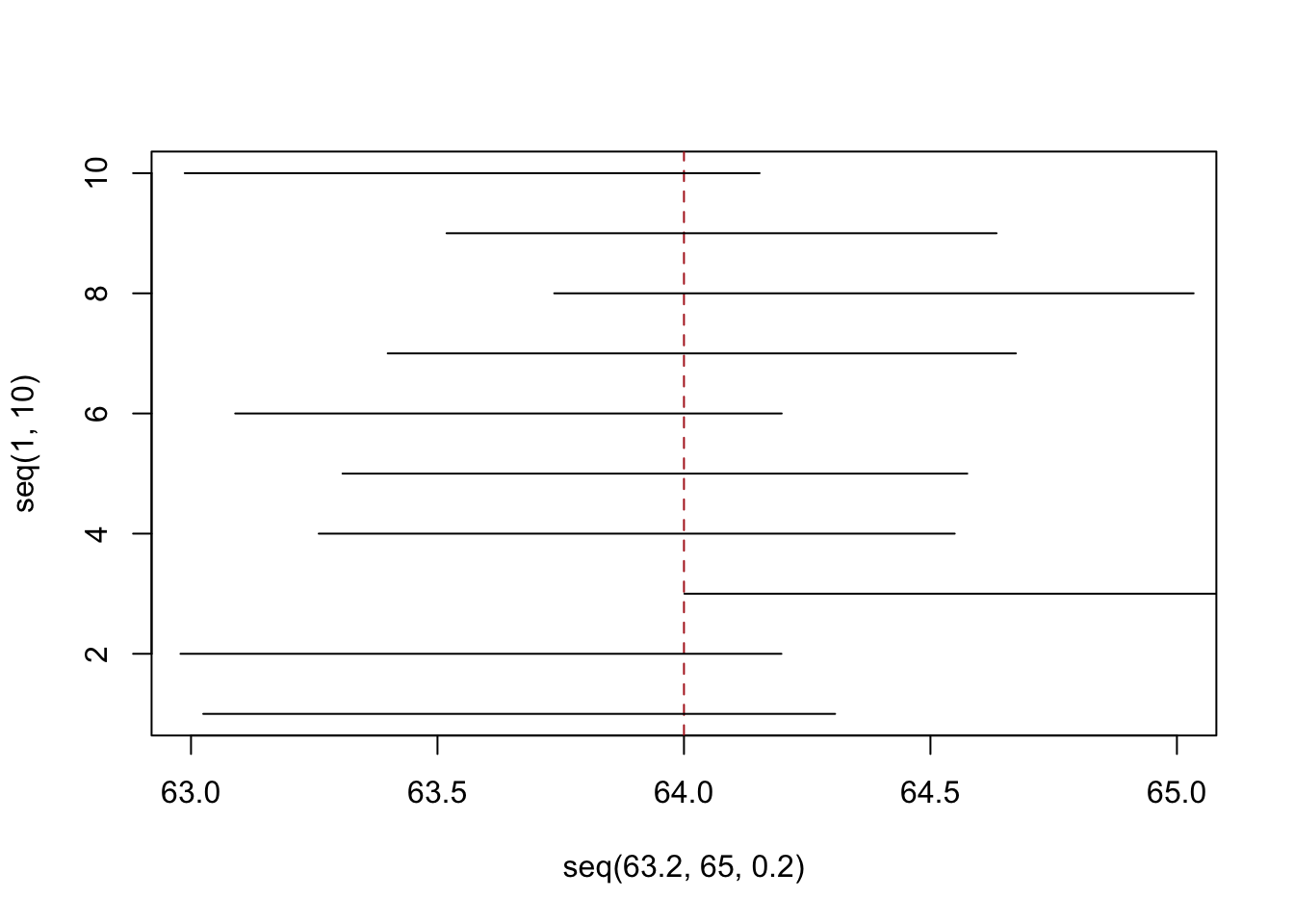
We expected that 0 or 1 of these confidence intervals would miss the true value, and indeed, one does.
Finally the standard error \(s/\sqrt{n}\) affects the width of the confidence interval. All else equal a larger \(s\) means a wider confidence interval. This makes sense! If your sample is more random, it is way harder to make a conclusion about where the true population parameter might be. For a larger \(n\) your confidence interval decreases. This is the law of large numbers! As the sample size increases the sample mean converges on the true population mean. As such, it makes sense that the confidence interval around any given sample mean will be smaller when \(n\) gets larger.
In all honesty I find confidence intervals minimally helpful, as they are more confusing than what is generally thought. Still: I got to teach them to you.
There is one additional (and very important) complication to what we have done so far. I have used thus far used the standard normal distribution to define the number of standard errors necessary to set a confidence interval. Let’s see what happens, however, if I use this method on a very small sample.
Let’s draw from the same distribution, but instead take a sample of 10 people. Again we are going to use the fact that 70% of the standard normal distribution is \(\pm1.04\) to define the bounds of a 70% confidence interval.
lower <- rep(NA,10)
upper <- rep(NA,10)

for(i in 1:10){
samp <- rnorm(10,64,3)
xbar <- mean(samp)
s <- sd(samp)
se <- s/sqrt(10)
lower[i] <- xbar - 1.04*se
upper[i] <- xbar + 1.04*se
}

plot( seq(63.2,65,.2),seq(1,10), type="n", xlim=c(63,65))
abline(v=64, lty=2, col="firebrick")
segments(lower, 1:10, upper, 1:10)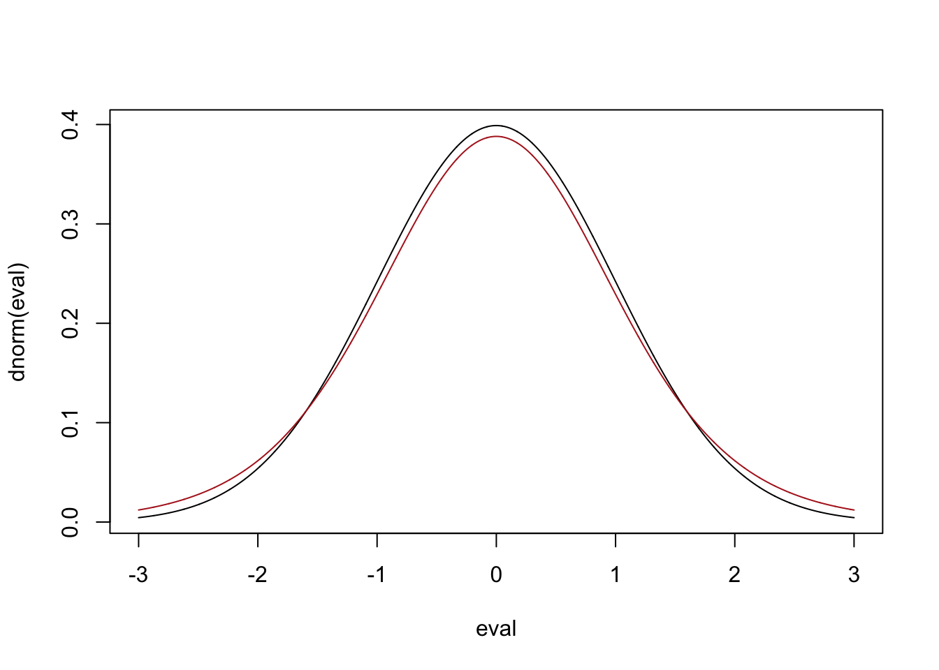
So far so good. As expected our confidence intervals are wider and 2 of them don’t contain the truth (we expect 3).
But! Let’s do this 10,000 times to see if it is true that 70% of constructed CIs contain the truth:
ci.contains <- rep(NA,10000)

for(i in 1:10000){
samp <- rnorm(10,64,3)
xbar <- mean(samp)
s <- sd(samp)
se <- s/sqrt(10)
lower <- xbar - 1.04*se
upper<- xbar + 1.04*se
ci.contains[i] <- lower<=64 & upper>=64
}
mean(ci.contains)
[1] 0.6801Whoops! Only 68% contain the truth. It’s close, but actually systematically wrong.
The very important reason is that when we are using the sample variance as a stand in for the population variance then the sampling distribution is not normally distributed.
When we were defining the sampling distribution before we found that the central limit theorem dictated that:
\[ \frac{\bar{X_n}-E[X]}{\sqrt{V[X]/n}} \sim N(0,1) \]
That if we took the sampling distribution of the sample means, subtracted off the truth and divided by the standard error we would be left with the standard normal distribution. This is equivalent to saying: the sampling distribution of the sample mean is normally distributed with mean \(\mu=E[X]\) and variance \(\sigma^2=V[X]/n\).
When we are using the sample standard deviation as a stand in for the population variance in the calculation of the standard error, however, the sampling distribution of the sample mean is:
\[ \frac{\bar{X_n}-E[X]}{s/\sqrt{n}} \sim t_{n-1} \]
Instead of collapsing to a standard normal, the sampling distribution is now \(t\) distributed with \(n-1\) degrees of freedom. The \(t\) distribution looks a lot like the normal distribution, but critically, it subtly changes its shape as \(n\) grows larger. At very low \(n\) the \(t\) distribution is shorter with fatter tails than the standard normal distribution.
Here is the t distribution with \(n-1=10-1=9\) degrees of freedom vs. the standard normal:
eval <- seq(-3,3,.001)
plot(eval, dnorm(eval), type="l")
points(eval, dt(eval,df=9), type="l", col="firebrick")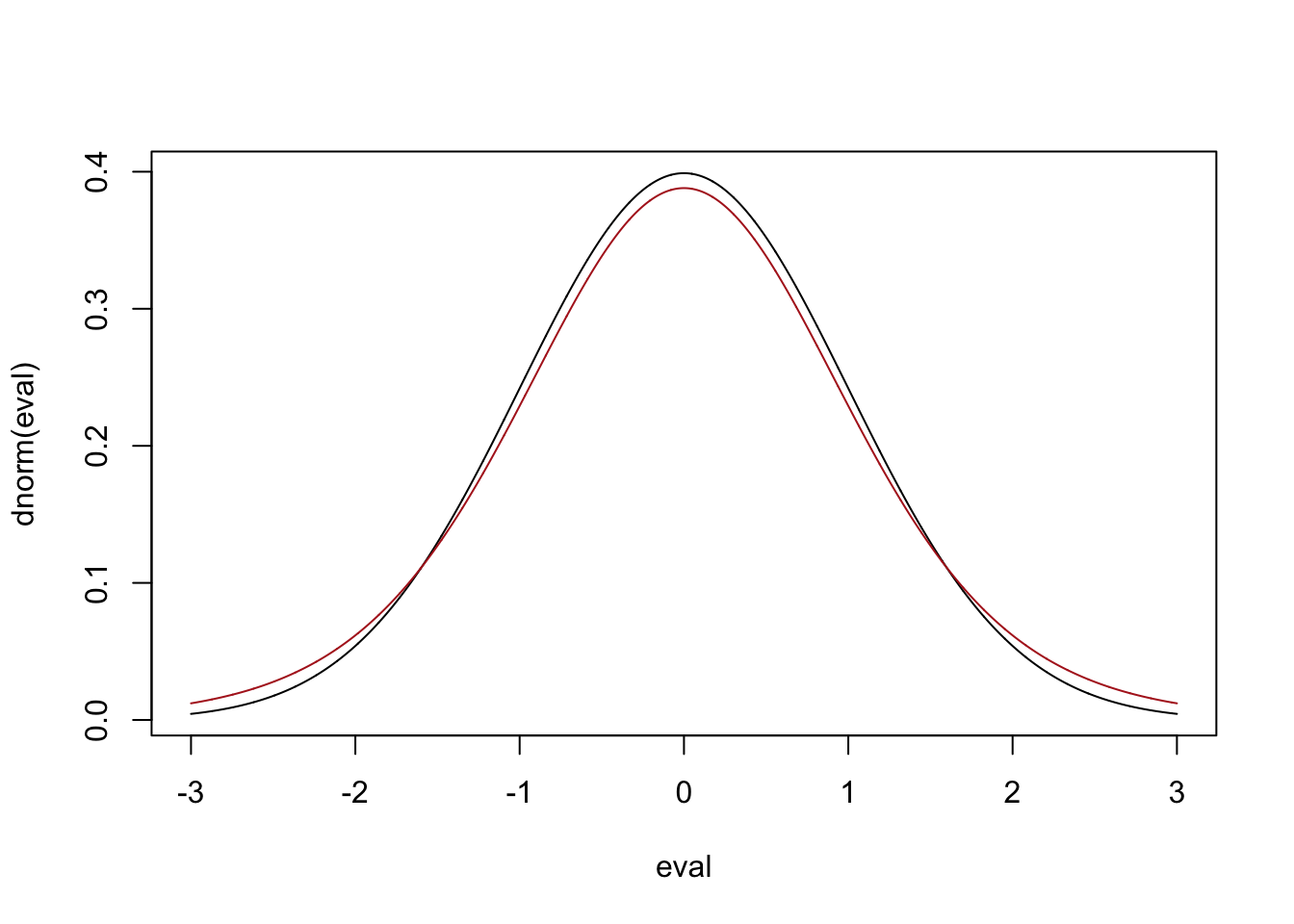
Because this t distribution is a different shape than the standard normal it means that when we are constructing a confidence interval using the sample variation as a stand in for the population variance we will get a different set of bounds based on the sample size.
To get the bounds for a 70% confidence interval:
#From the standard normal
qnorm(.15)
[1] -1.036433#Using the t distribution
qt(.15, df=9)[1] -1.099716And now let’s use that to define our bounds and see if 70% of confidence intervals contain the truth:
ci.contains <- rep(NA,10000)

for(i in 1:10000){
samp <- rnorm(10,64,3)
xbar <- mean(samp)
s <- sd(samp)
se <- s/sqrt(10)
lower <- xbar - 1.10*se
upper<- xbar + 1.10*se
ci.contains[i] <- lower<=64 & upper>=64
}
mean(ci.contains)
[1] 0.6974Yes! So the T distribution is what you must use to define a confidence interval if you are using the sample variance as a stand in for the population variance.
OK: but why did using the standard normal work when we had a sample size of 100? This is because the \(T\) distribution converges on the standard normal distribution as n gets larger than, like, 30:
eval <- seq(-3,3,.001)
plot(eval, dnorm(eval), type="l")
points(eval, dt(eval,29), type="l", col="firebrick")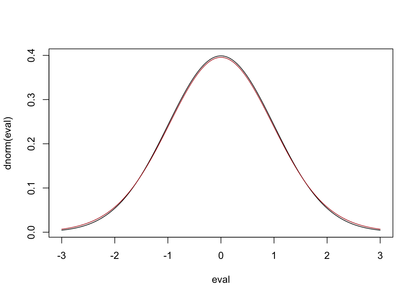
So the \(t\) distribution only gives you a different answer than the standard normal for \(n\)’s that are under 30.
That being said: in this class you must use the t distribution if you are calculating a confidence interval or doing a hypothesis test on a sample of data and subbing in the sample variance for the population variance. Even though it “doesn’t matter” that is the distribution of the sampling distribution under these conditions.
We now have the tools to make an inferential claim from a single sample: use the sample variance as a stand-in for the population variance, center a sampling distribution on our sample mean, and use the \(t\) distribution to define bounds that contain the true population parameter some percentage of the time. That is a confidence interval.
The other half of statistical inference asks the mirror-image question. Instead of “given my sample, where does the truth plausibly lie?”, we ask “given a specific claim about the truth, is my sample consistent with it?” That is a hypothesis test, and it’s what we turn to next. T
This is technically not true. I will explain below why this is not technically true and why I don’t care. If you are someone not in my class reviewing this textbook and got mad reading this sentence: I know that it’s wrong.↩︎