choose(52,5)[1] 2598960Problem Set Due Wednesday September 25th at 7pm on Canvas.
You will hand in a .Rmd file and a knitted html output.
I have provided the raw RMD of this problem set you can use as a template for answering.
(a) In a game of poker each player is dealt 5 cards from a 52 card deck. How many different 5 card poker hands can be generated from a 52 card deck? (Hint: Is this a permutation or a combination?).
choose(52,5)[1] 2598960This is a combination because the order of poker hands doesn’t matter
(b) There are 4 suits in a card deck, each consisting of 13 cards. A “flush” is a poker hand where all 5 cards are of the same suit. Calculate the probability of being dealt a flush. (Hint: You first need to count all the ways you can make a 5 card hand using only cards from one suit.)
#How many ways can you have a flush within a suit of 13 cards?
choose(13,5)
[1] 1287#There are 4 suits so
1287*4[1] 5148#Out of all possible hands
(choose(13,5)*4)/choose(52,5)[1] 0.001980792The odds of a flush are about .2%.
(c) Simulate the answer to question (b) using R. Run a loop 100000 times that draws 5 cards from a deck of 52, where there are 4 suits with 13 cards each. Note, that we don’t care which cards are which within a suit. We just need 13 hearts, 13 diamonds, 13 clubs, 13 spades. How often are you dealt a flush? (Hint: to see if all the cards in my hand were of the same suit I started with the unique() command.)
#Set up
deck<- c(rep("hearts",13),rep("diamonds",13), rep("clubs",13), rep("spades",13))

#Sample WITHOUT REPLACEMENT
hand <- sample(deck,5,replace=F)

#Test to see if all of the cards are from the same suit

length(unique(hand))==1
[1] FALSE#No they are not
#Loop and record successes:
flush <- rep(NA, 100000)
for(i in 1:length(flush)){
hand <- sample(deck,5,replace=F)
flush[i] <- length(unique(hand))==1
}
prop.table(table(flush))flush
FALSE TRUE
0.99817 0.00183 We get a approximarely similar .2% via simulation.
(d) A manufacturer of code-based locks comes to you worried that the codes on his lock are too easy to guess. He tells you that his locks have a dial with 10 numbers and the codes are 3 digits long. Like most locks, the numbers in the code cannot repeat and the order of the numbers matters. Calculate the probability of guessing this code using both math and simulation. For the simulation, run the loop 1 million times.
#A lock with 10 numbers and a code length of 3

#This gives the number of combinations:
choose(10,3)
[1] 120#Need to multiply by 3! to get permutations
1/(choose(10,3)*factorial(3))[1] 0.001388889#The probability of guessing this lock is actually quite low at .014%
#Through simulation
set.seed(19104)
dial <- seq(1,10,1)
prime <- sample(dial,3, replace=F)
result <- rep(NA, 1000000)
for(i in 1:length(result)){
result[i] <- all(sample(dial,3, replace=F)==prime)
}
prop.table(table(result))result
FALSE TRUE
0.998599 0.001401 #We get approximately the same result through simulationBoth the simulation and math routes give a similar answer that any given guess has a .01% probability of being correct.
(e) To help this manufacturer we want to determine if it’s more effective to manufacture a bigger dial or to require the user to use a longer code. Using R to simulate each possibility 1 million times, make two graphs. For the first graph, determine the probability of guessing a code with dial sizes from 10 to 30 numbers and a 3 digit code. For the second graph, determine the probability of guessing a code with a dial size of 10, but code lengths from 3-10 numbers long. What do you find?
#Reuse our code but make the dial length a variable
set.seed(19104)

lengths <- seq(10,30,1)
prob.guess <- rep(NA, length(lengths))

for(j in 1:length(lengths)){
  dial <- seq(1,lengths[j],1)
  prime <- sample(dial,3, replace=F)
  result <- rep(NA, 1000000)

  for(i in 1:length(result)){
    result[i] <- all(sample(dial,3, replace=F)==prime)
  }
 prob.guess[j] <- prop.table(table(result))[2]
}

plot(lengths, prob.guess, pch=16, type="b", ylab="Probability of Guessing Right",
     xlab="Dial Sizes",
     main="Probability of Correct Guess with Code Length 3 and Varying Dial Size")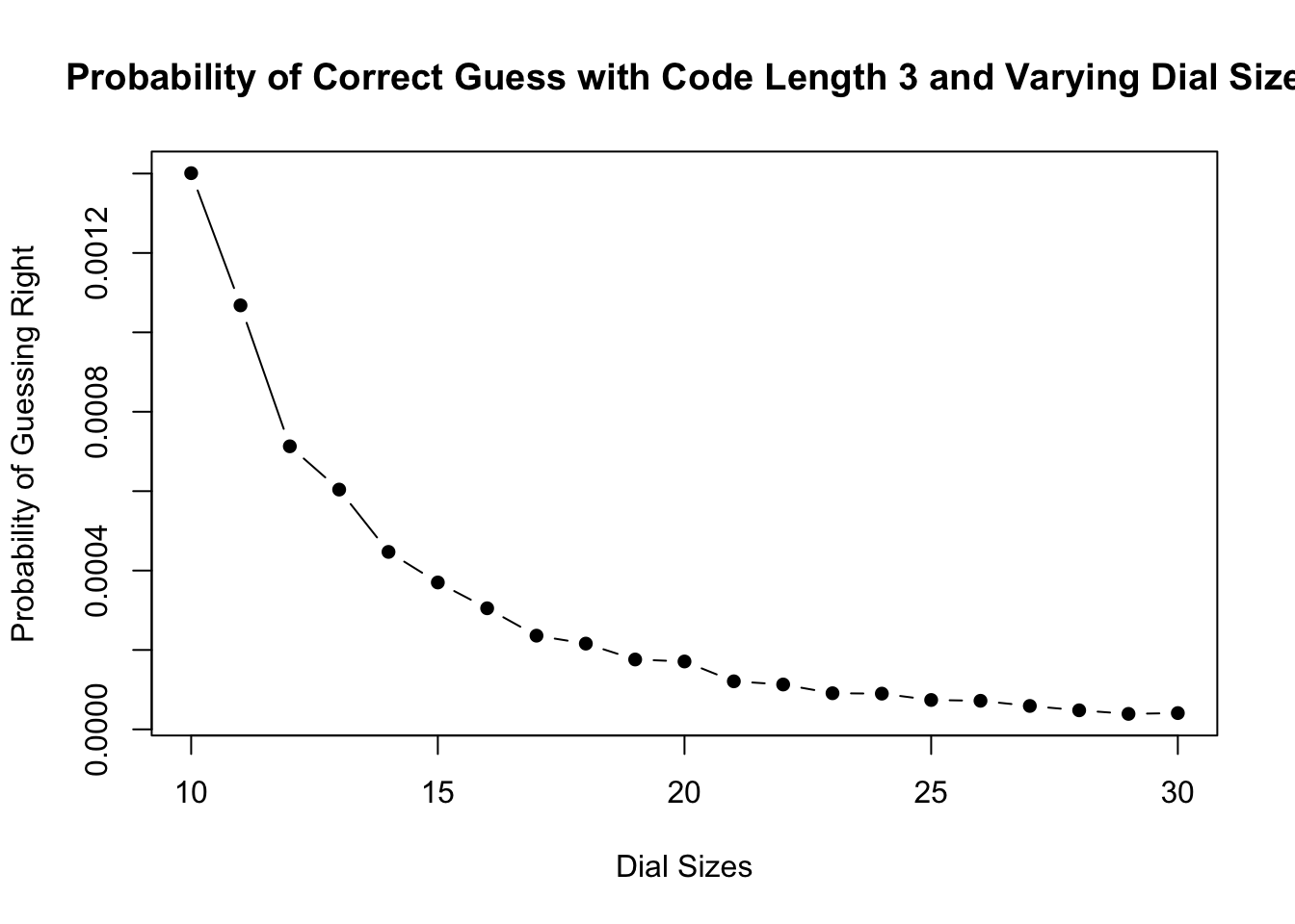
#Reuse our code but make the dial length a variable
set.seed(19104)

codes <- seq(3,10,1)
prob.guess <- rep(NA, length(codes))

for(j in 1:length(codes)){
  dial <- seq(1,10,1)
  prime <- sample(dial,codes[j], replace=F)
  result <- rep(NA, 1000000)

  for(i in 1:length(result)){
    result[i] <- all(sample(dial,codes[j], replace=F)==prime)
  }
 prob.guess[j] <- mean(result)
}

plot(codes, prob.guess, pch=16, type="b", ylab="Probability of Guessing Right", xlab="Code Length",
     main="Probability of Correct Guess with Dial Size 10 and Varying Code Length")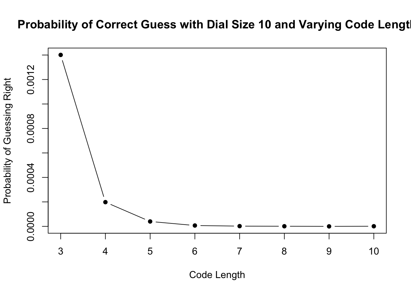
As would be expected, reducing both increasing the dial size and increasing the code length cause the probability of any particular combination being a correct guess to decrease. That being said, it appears that increasing the code length has a much more dramatic effect than increasing the dial size.
For example, with a code of length 3 increasing the dial size from 10 to 11 changes the number of permutations by:
choose(11,3)*factorial(3) - choose(10,3)*factorial(3)[1] 270While changing the code length from 3 to 4 for a dial length of 10 increases the number of permutations by:
choose(10,4)*factorial(4) - choose(10,3)*factorial(3)[1] 4320Factorials, man!
The dataset apps is (fake) data on 100,000 college applicants. We have indicator (dummy) variables for high.sat (whether they scored high on the SAT or not), admit (whether they were admitted to the college or not), and high.performer (whether they will perform highly in college or not).
apps <- rio::import("https://github.com/marctrussler/IIS-Data/raw/refs/heads/main/PS1CondProb.Rds", trust=T)mean(apps$high.performer)[1] 0.50195Just over 50% of the applicants are high performers.
#High performance given low SAT
mean(apps$high.performer & apps$high.sat==0)/mean(apps$high.sat==0)
[1] 0.4031923#High performance given high SAT
mean(apps$high.performer & apps$high.sat)/mean(apps$high.sat)[1] 0.6011828Amongst all applicants, the probability of being a high performer with a low SAT score is 40%, and the probability of being a high performer with a high SAT score is 60%. SAT scores predict success.
#High performance given low SAT and admitted
mean(apps$high.performer & apps$high.sat==0 & apps$admit)/mean(apps$high.sat==0 & apps$admit)
[1] 0.9459232#High performance given high SAT
mean(apps$high.performer & apps$high.sat & apps$admit)/mean(apps$high.sat & apps$admit)[1] 0.7476252The probability of being a high performer with a low SAT score among admitted students is 94%. The probability of being a high performer with a high SAT score among the admitted is 74%. So among admitted students SAT score has a negative effect on performance: the higher the SAT score the lower the performance.
This is a classic example of Berkson’s paradox where two desirable traits (here test performance and college performance) appear negatively related in a selected sample while they are positively related in the full population. Why does this occur? It does so because selection isn’t random. In particular, by design we do not get low-SAT, low-perfoming students admitted into college. Among the low-SAT students we only get high performing students. Put another way: in order to get into college with a low SAT score you must excel elsewhere. That means that conditional on getting in, a low SAT student is extremely likely to do well because they have other talents that allowed them to succeed. High SAT students get in on scores alone, but factoring in the other intangible factors that lead to success this group is a mix of true high performers, and low perfomers who are just good at tests. This creates the (false!) negative relationship that we see.
Another example is that height and scorign are negatively correlated in the NBA. Tall people are allowed into the NBA because they are tall, but once there there other skills may cause them to score less (Shawn Bradley: 7’6” and 8.1 points a game). But a short player only gets into the NBA if they are immensely skilled (my friend and fellow Canadian Steve Nash, 6’3” 14.3 points per gamge), and we don’t observe any short players who are bad.
Consider the following probability mass function of a random variable, \(K\):
\[ f(K) = p(K=k) = \begin{cases} \frac{1}{6} \text{ if } 1\\ \frac{1}{3} \text{ if } 2\\ \frac{1}{3} \text{ if } 4\\ \frac{1}{6} \text{ if } 10\\ \end{cases} \]
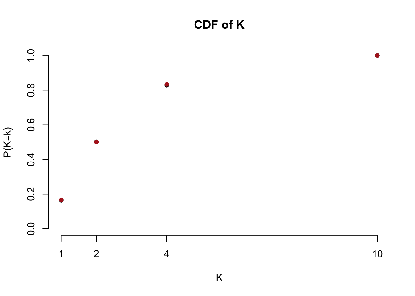
The CDF of K is:
\[ F(K) = p(K < k) = \begin{cases} 0 \text{ if } K <1\\ \frac{1}{6} \text{ if } 1\leq k <2\\ \frac{1}{2} \text{ if } 2\leq k <4\\ \frac{5}{6} \text{ if } 4\leq k <10\\ 1 \text{ if } 10\leq k\\ \end{cases} \]
The expected value of K is:
\[ \begin{align} E[K] = &\sum k*f(k)\\ = &1*\frac{1}{6} + 2*\frac{1}{3} + 4*\frac{1}{3} + 10*\frac{1}{6}\\ = & 3.833\\ \end{align} \]
\[ \begin{align} E[X^2]= &1^2*\frac{1}{6} + 2^2*\frac{1}{3} + 4^2*\frac{1}{3} + 10*^2\frac{1}{6}\\ = &23.5\\ E[X]^2 = &3.83^2 = 14.6689\\ V[K] = &E[X^2] - E[X]^2\\ = &23.5-14.6689\\ = & 8.83 \end{align} \]
set.seed(19104)
#Option 1:
coin <- c(rep(1,10), rep(2,20), rep(4,20), rep(10,10))
samp <- sample(coin, 10000, replace=T)

#Option 2 (slightly cleaner)
samp <- sample(c(1,2,4,10),10000, prob=c((1/6), (1/3), (1/3), (1/6)), replace = T)

mean(samp)
[1] 3.864var(samp)[1] 8.992203#Both Matchcumsum() function.#PMF
values <- sort(unique(samp))
probs <- prop.table(table(samp))
true.probs <- c((1/6), (1/3), (1/3), (1/6))
plot(values, probs, pch=16, ylim=c(0,.4), axes=F,
xlab="K", ylab="P(K=k)",
main="PMF of K", col="darkblue")
axis(side=2)
axis(side=1, at=c(1,2,4,10))
points(values, true.probs, col="firebrick", pch=16)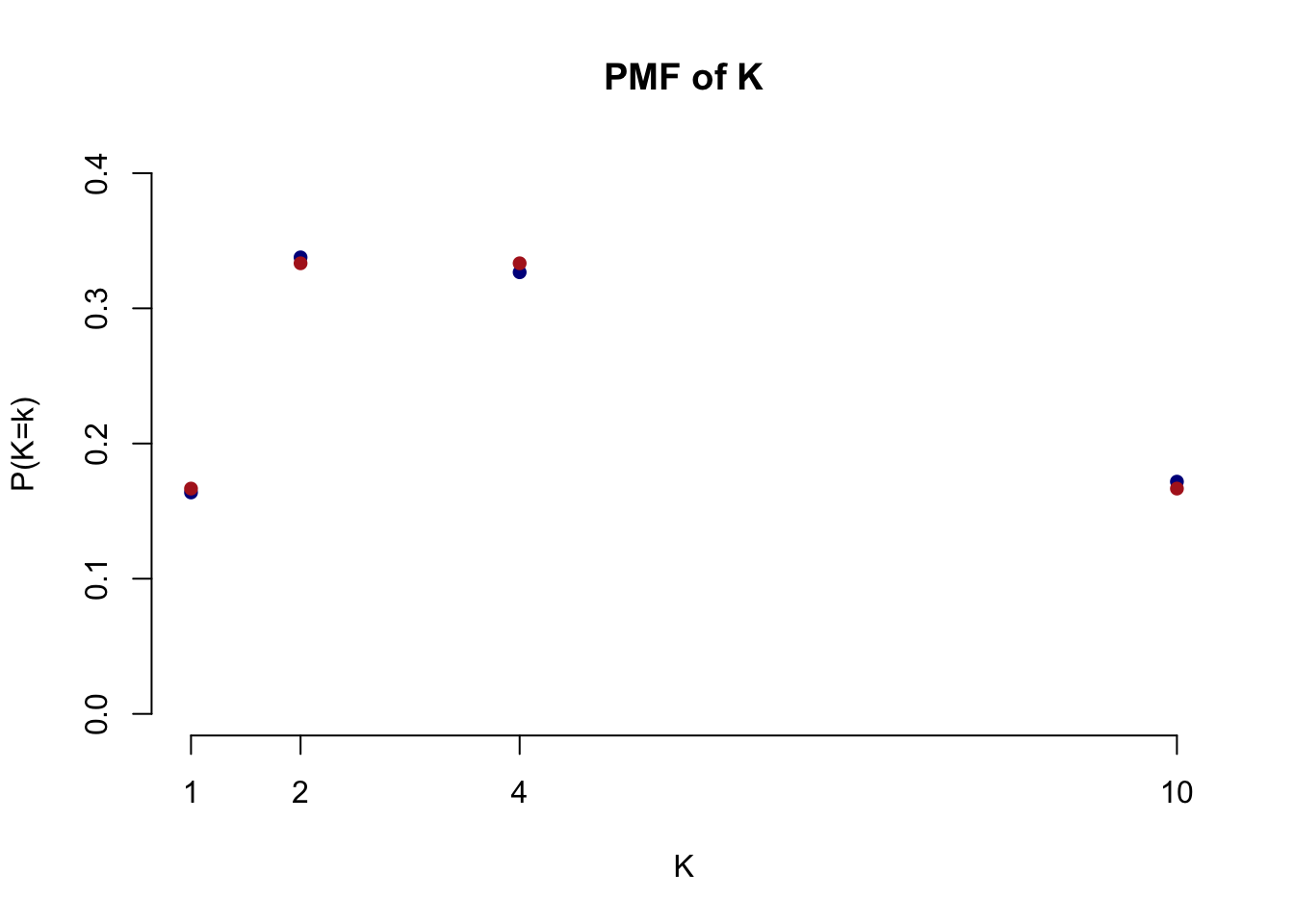
#CDF

probs.cdf <- cumsum(probs)
true.probs.cdf <- cumsum(true.probs)

plot(values,cumsum(probs), pch=16, ylim=c(0,1), axes=F,
     xlab="K", ylab="P(K=k)",
     main="CDF of K")
axis(side=2)
axis(side=1, at=c(1,2,4,10))
points(values, true.probs.cdf, col="firebrick", pch=16)