set.seed(19104)
#X exists:
x <- rnorm(100, mean=50, sd=3)
#Y data generating process:
y <- 4 + 3*x + rnorm(100,mean=0, sd=2)
plot(x,y)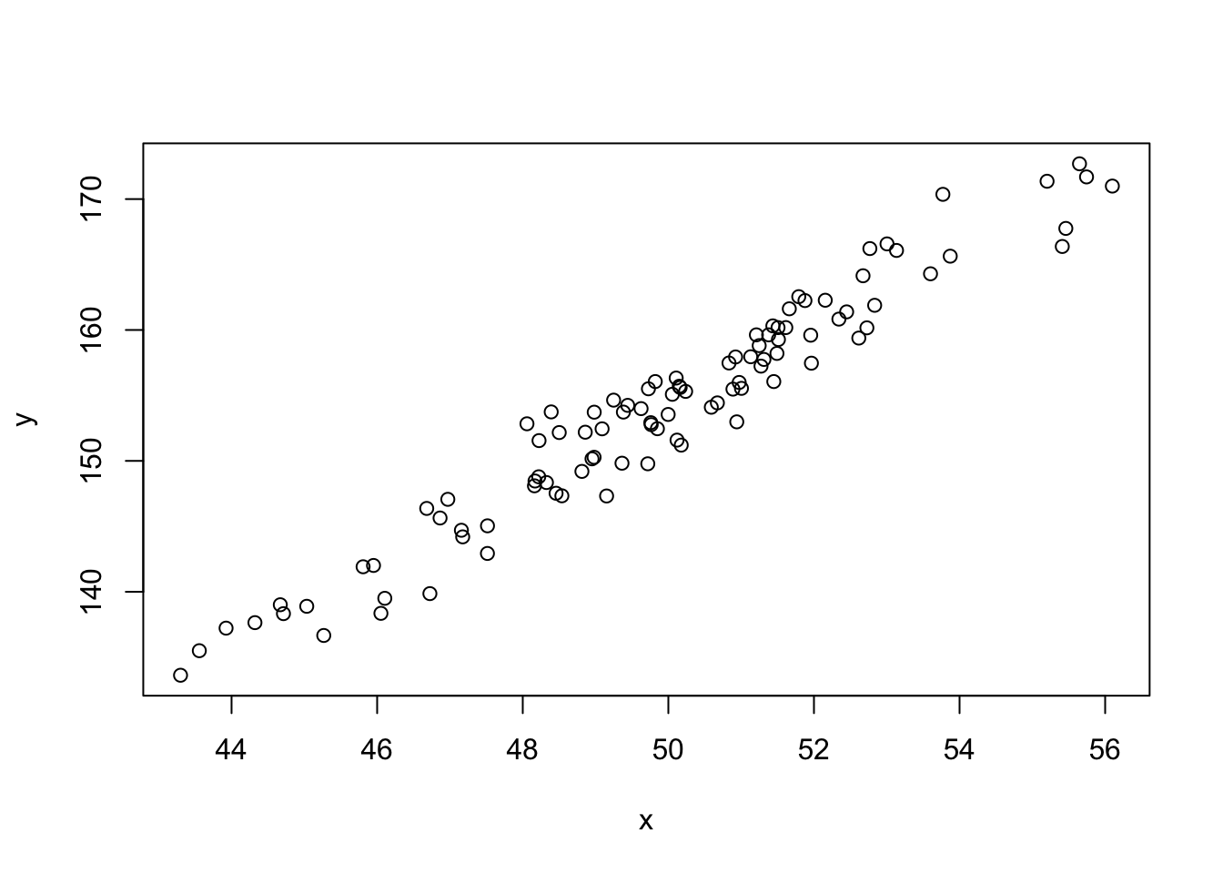
#Everytime we runw we get something new📄 Download the R code from this chapter
📝 Download the class handout for this chapter
You can run regression on any set of numerical variables, but that does not mean that your regression is giving you the “right” answer, or the true relationship between the independent and dependent variables in the population.
In order for your regression to be outputting the “right” answers the regression must satisfy 5 criteria called the “Gauss-Markov Assumptions”.
Before getting there, I want to talk about one twist to the regression equation, which we have defined as:
\[ \hat{y} = \hat{\alpha} + \hat{\beta} X_i \]
As we have discussed, this equation defines the regression line. You can input an x and it will output a the y-level of the regression line at that point.
We can also write the following equation
\[ y_i = \hat{\alpha} + \hat{\beta} x_i + \hat{u}_i \]
The middle bit \(\alpha + \beta x_i\) is the same, and we know this produces the regression line. But notice that the left hand side is no longer set equal to \(\hat{y}\) but instead to \(y_i\). In other words, this is the equation which tells you, for a given x, what does the actual y value equal? To get from the regression line to the actual y value, we need to add back on the residual which in the sample is \(u_i\). So this equation says, for our sample, this is the relationship between x’s and y’s.
We can also think about this same equation existing in the population:
\[ Y_i = \alpha + \beta X_i + \epsilon_i \]
When we talk about the population we get rid of the hats (which denote that something is an estimate) and also change \(u\) to \(\epsilon\). What we are effectively defining here is the data generating process. How do y’s get produced by x’s? Well there is some sort of population level intercept and slope, but those aren’t purely deterministic. To each point is added some amount of error, \(\epsilon\), which generates our final data. We could literally generate data using a similar equation (and this is similar to your problem set):
set.seed(19104)
#X exists:
x <- rnorm(100, mean=50, sd=3)
#Y data generating process:
y <- 4 + 3*x + rnorm(100,mean=0, sd=2)
plot(x,y)
#Everytime we runw we get something newThinking this way about the regression equation as a “data generating process”, we can think about the GM assumptions.
The Gauss-Markov Assumptions are:
We are going to talk about these a bit out of order.
The first, that X has full rank, is saying that one variable cannot be a linear combination of others. We actually just saw an example of this when we were making categorical variables. There we saw that if we had an exhaustive set of categories OLS must drop one in order to actually compute. The only other situation that this will happen is if you try to regress a variable that has no variation. A variable with no variation is a linear transformation of the intercept, so that won’t work!
The first assumption is not really one you have to think about because R will literally not run a regression that violates this, as we saw above.
Similarly, if you try to run a regression with an independent variable that has no variation:
y <- rnorm(100,50,25)
x <- rep(0,100)
plot(x,y)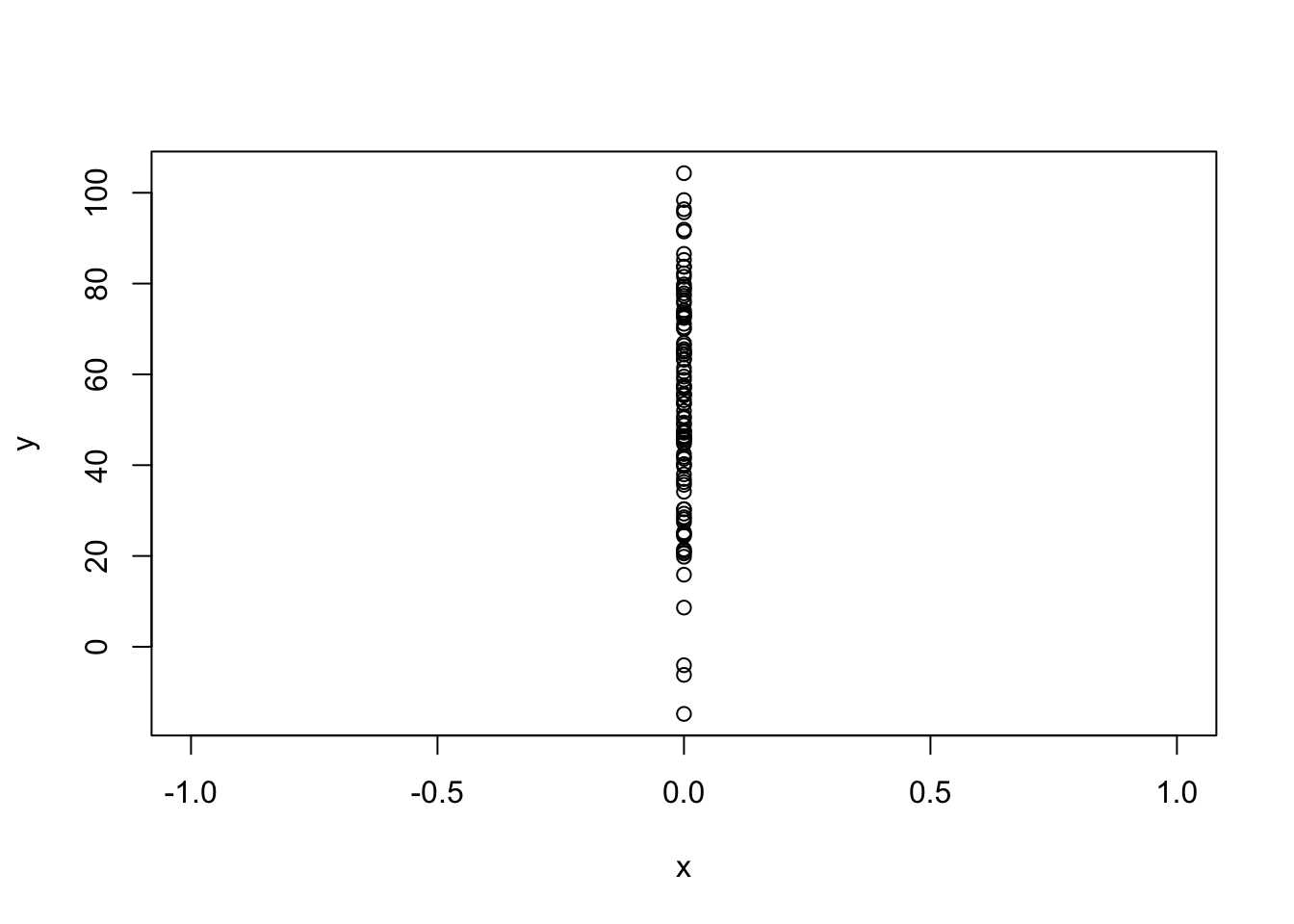
lm(y ~ x)
Call:
lm(formula = y ~ x)

Coefficients:
(Intercept)            x
53.46 NA Jumping around, the 5th OLS assumption that \(E[\epsilon_i|X] = 0\) is talking about causality. This is sometimes thought of as an extra or “bonus” assumption that \(\beta\) actually represents the true effect of X on Y. One way we think about that is saying that the errors \(\epsilon\) are uncorrelated with other factors. You can just think of this as: there are no confounding variables.
m <- lm(percent.transit.commute ~ median.income, data=acs)Assumptions 3 and 4 are a bit more important, as they talk about whether we can trust the standard errors being produced. Both of these assumptions are about each point being independent from all other points. If each point is independent from all other points then it must also be the case that each points error term \(\epsilon\) is independent from all other points. A couple of things break this.
Assumption 3 says that, conditional on x, the squared error term must be equal to \(\sigma^2\). Less important here is what sigma squared is, and more important is that this is saying that the error must be constant across levels of X.
Have a look at these two graphs:
#Homoskedastic Errors
x <- runif(100, min=0, max=100)
y <- 2 + 3*x + rnorm(100, mean=0, sd=15)

plot(x,y)
abline(lm(y~x), col="firebrick" ,lwd=2)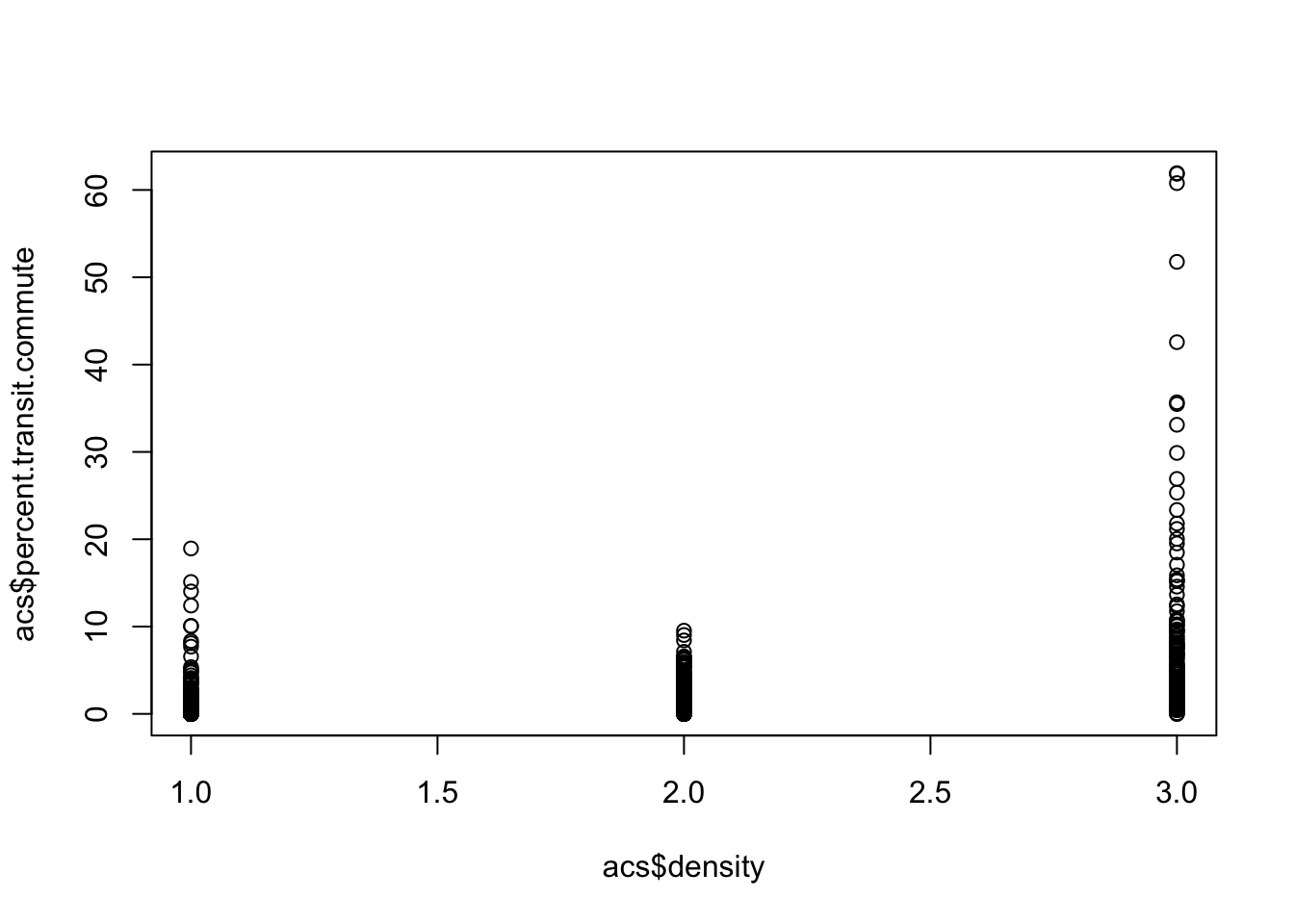
#Heteroskedastic Errors
x <- runif(100, min=0, max=100)
y <- 2 + 3*x + rnorm(100, mean=0, sd=x*2)

plot(x,y)
abline(lm(y~x), col="firebrick" ,lwd=2)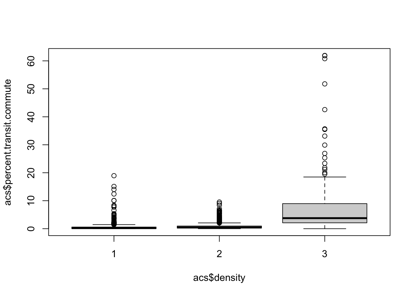
In the second graph the errors are not constant across levels of X. These are heteroskedastic errors. The consequence of these is that the estimated standard error on beta will be wrong.
We can show that via simulation
betas <- rep(NA,10000)
ses <- rep(NA,10000)

for(i in 1:10000){
x <- runif(100, min=0, max=100)
y <- 2 + 3*x + rnorm(100, mean=0, sd=x*2)
m <- lm(y ~ x)

betas[i] <- coef(m)["x"]
ses[i] <- sqrt(vcov(m)["x","x"])
}

#Empirical standard error
sd(betas)
[1] 0.4423603#Average calculated standard errors in samples
mean(ses)[1] 0.399791How to do we diagnose and address heteroskedasticity?
library(AER)
data("CASchools")
head(CASchools)
district school county grades students teachers
1 75119 Sunol Glen Unified Alameda KK-08 195 10.90
2 61499 Manzanita Elementary Butte KK-08 240 11.15
3 61549 Thermalito Union Elementary Butte KK-08 1550 82.90
4 61457 Golden Feather Union Elementary Butte KK-08 243 14.00
5 61523 Palermo Union Elementary Butte KK-08 1335 71.50
6 62042 Burrel Union Elementary Fresno KK-08 137 6.40
calworks lunch computer expenditure income english read math
1 0.5102 2.0408 67 6384.911 22.690001 0.000000 691.6 690.0
2 15.4167 47.9167 101 5099.381 9.824000 4.583333 660.5 661.9
3 55.0323 76.3226 169 5501.955 8.978000 30.000002 636.3 650.9
4 36.4754 77.0492 85 7101.831 8.978000 0.000000 651.9 643.5
5 33.1086 78.4270 171 5235.988 9.080333 13.857677 641.8 639.9
6 12.3188 86.9565 25 5580.147 10.415000 12.408759 605.7 605.4#Creating Variables
CASchools$STR <- CASchools$students/CASchools$teachers
summary(CASchools$STR) Min. 1st Qu. Median Mean 3rd Qu. Max.
14.00 18.58 19.72 19.64 20.87 25.80 CASchools$score <- (CASchools$read + CASchools$math)/2
summary(CASchools$score) Min. 1st Qu. Median Mean 3rd Qu. Max.
605.6 640.0 654.5 654.2 666.7 706.8 dat <- CASchoolsdat$esl <- dat$english
#lm(math ~ esl)Before we plot this to assess hetero/homoskedasticity let’s think through what is likely to be the case. Do we expect more variation in math scores when esl is high/low?
Probably, yes. My expectation is that schools with a low number of esl kids will be in all sorts of neighborhoods with all sorts of different levels of funding, family income etc.
So I expect a lot of variation in math scores in these types of schools. Schools with a high number of esl kids will all be in similar types of neighborhoods so I expect a bit less variation in math scores in these schools.
Note that we’re not talking about the relationship between esl and math scores, but how the random variance in math changes across levels of esl.
Further, while we have tools to diagnose heteroskedasticity, part of what you do will be using your theoretical knowledge of cases to determine whether it is likely to be a problem. This is what I did here with my deep knowledge of the California school system (kidding! I cheated and looked at the data first…)
Let’s take a look at what we see.
plot( dat$esl, dat$math)
abline(lm(dat$math ~ dat$esl), col="firebrick", lwd=2)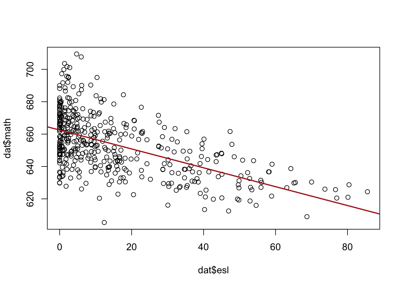
This seems to reflect our prediction, in general there seems to be a lot more variation in math scores when esl is lower, and less when esl is higher.
There is a specific test for heteroskedasticity beyond what we can see with our eyes:
library(lmtest)
m <- lm(math ~ esl, data=dat)
bptest(m)
    studentized Breusch-Pagan test

data:  m
BP = 12.084, df = 1, p-value = 0.0005085
This test will be statistically significant if heteroskedasticity is present. Here we reject the null hypothesis of homoskedasticity.
How can we fix this?
Well, one way to fix heteroskedasticity is to better model the reasons for higher variance in some cases.
We think that there is more unmodeled variance at the low end of esl. In other words schools without a lot of english as a second language children come from all different types of places. If we add variables that explain math scores among that group better heteroskedasticity will be reduced.
So, for example, if we add to our regression other variables which help us determine what sort of schools these are…
m <- lm(math ~ esl + lunch + calworks + income, data=dat)
summary(m)
Call:
lm(formula = math ~ esl + lunch + calworks + income, data = dat)

Residuals:
     Min       1Q   Median       3Q      Max
-30.8808  -6.6403  -0.0207   5.8995  30.0311

Coefficients:
             Estimate Std. Error t value Pr(>|t|)
(Intercept) 660.25387    2.47171 267.124  < 2e-16 ***
esl          -0.14893    0.03831  -3.887 0.000118 ***
lunch        -0.32979    0.04215  -7.825 4.26e-14 ***
calworks     -0.11171    0.06657  -1.678 0.094090 .
income        0.76129    0.09542   7.979 1.46e-14 ***
---
Signif. codes:  0 '***' 0.001 '**' 0.01 '*' 0.05 '.' 0.1 ' ' 1

Residual standard error: 9.928 on 415 degrees of freedom
Multiple R-squared:  0.7224,    Adjusted R-squared:  0.7198
F-statistic: 270 on 4 and 415 DF, p-value: < 2.2e-16bptest(m)
    studentized Breusch-Pagan test

data:  m
BP = 7.4826, df = 4, p-value = 0.1125
We no longer have a heteroskedastic regression.
The other way to deal with heteroskedasticity is to employ Hubert-White (or simply “robust”) standard errors.
For this we need the sandwich package
library(sandwich)
library(lmtest)
m <- lm(math ~ esl, data=dat)
robust.vcov <- vcovHC(m, type="HC1")
coeftest(m, vcov=robust.vcov)
t test of coefficients:

              Estimate Std. Error t value  Pr(>|t|)
(Intercept) 662.539315   1.046782 632.929 < 2.2e-16 ***
esl          -0.583245   0.033671 -17.322 < 2.2e-16 ***
---
Signif. codes: 0 '***' 0.001 '**' 0.01 '*' 0.05 '.' 0.1 ' ' 1Assumption 4 talks about “auto-correlation”. This has the same problem of breaking the assumption that the errors of one data point are independent from others, but here it is because that points are related to one another in some un-modeled way. This is almost always due to time or to clusters.
First let’s think about time:
Here is quarterly American GDP since the year 2000:
gdp <- import("https://github.com/marctrussler/IIS-Data/raw/main/GDP.csv")
gdp <- gdp[213:307,]

plot(gdp$DATE, gdp$GDP)
abline(lm(gdp$GDP ~ gdp$DATE), col="firebrick", lwd=2)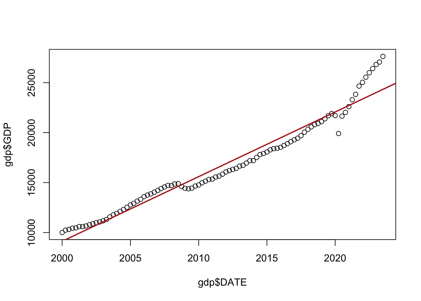
Now, ignoring the fact there that this red line doesn’t do a great job of fitting the data, the problem here is that the errors being made from point to point are not independent from one another.
Let’s look at the relationships between the date and the residuals from that regression:
gdp$residuals <- residuals(lm(gdp$GDP ~ gdp$DATE))
plot(gdp$DATE, gdp$residuals)
abline(h=0)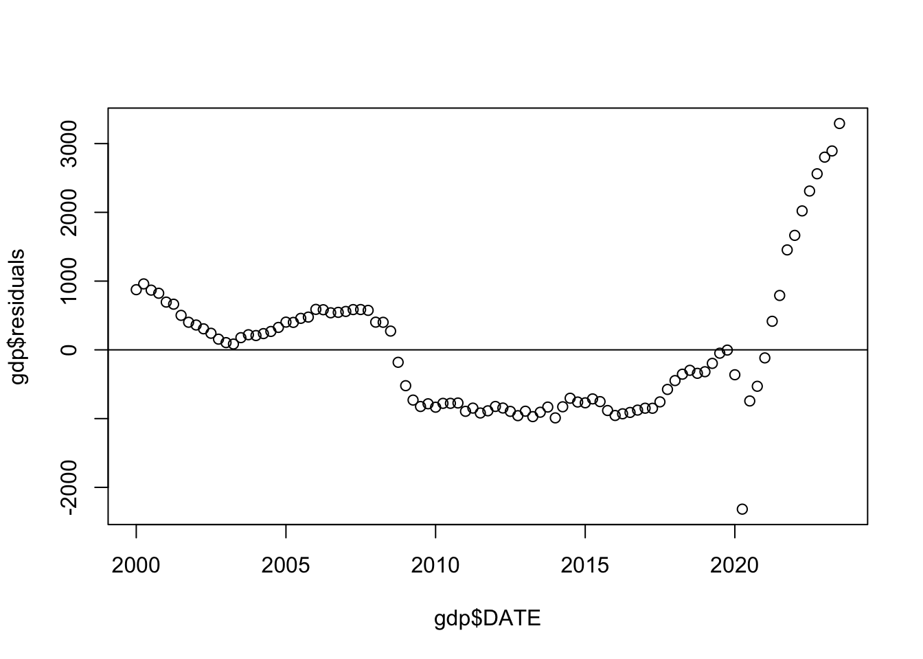
What we want to think about is that if there are two adjacent points than a lot of the time knowing the residual of one point will tell you what the residual of the neighboring point is. There are some exceptions here (like the 2nd quarter of 2020!), but in general if you tell me the error of one point I can make a good guess at the error of it’s neighbor.
For comparison, here is what this same plot looks like when things are fine (from the data we created abo:
x <- runif(100, min=0, max=100)
y <- 2 + 3*x + rnorm(100, mean=0, sd=15)
resid <- residuals(lm(y~x))
plot(x,resid)
abline(h=0)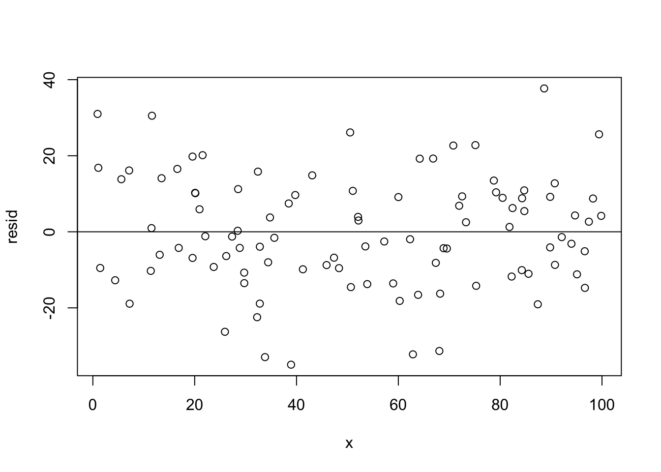
Here the error on one point doesn’t really tell you anything about its neighbors.
How do we deal with time-based autocorrelation? Run! It’s very hard to deal with and is the focus of full courses. For right now it’s enough to know that this sort of pattern runs counter to the assumption of OLS.
The other situation that breaks the assumptions of OLS is when your data comes from clusters.
Using the ACS data, let’s look at the relationship between the percent of people with a college degree and median income, but only for counties in either NY and MS. (These states chosen to be the most different possible.)
Here is the relationship at the baseline:
head(acs) V1 county.fips county.name state.full state.abbr state.alpha state.icpsr
1 1 1055 Etowah County Alabama AL 1 41
2 2 1133 Winston County Alabama AL 1 41
3 3 1053 Escambia County Alabama AL 1 41
4 4 1001 Autauga County Alabama AL 1 41
5 5 1003 Baldwin County Alabama AL 1 41
6 6 1005 Barbour County Alabama AL 1 41
census.region population population.density percent.senior percent.white
1 south 102939 192.30800 18.33804 80.34856
2 south 23875 38.94912 21.05550 96.33927
3 south 37328 39.49123 17.34891 61.87045
4 south 55200 92.85992 14.58333 76.87862
5 south 208107 130.90190 19.54043 86.26620
6 south 25782 29.13214 17.97378 47.38189
percent.black percent.asian percent.amerindian percent.less.hs
1 15.7491330 0.7179009 0.7295583 15.483020
2 0.3769634 0.1298429 0.3895288 21.851723
3 31.9331333 0.3616588 3.8496571 18.455613
4 19.1394928 1.0289855 0.2880435 11.311414
5 9.4970376 0.8072770 0.7313545 9.735422
6 47.5758281 0.3723528 0.2792646 26.968580
percent.college unemployment.rate median.income gini median.rent
1 17.73318 6.499382 44023 0.4483 669
2 13.53585 7.597536 38504 0.4517 525
3 12.65935 13.461675 35000 0.4823 587
4 27.68929 4.228036 58786 0.4602 966
5 31.34588 4.444240 55962 0.4609 958
6 12.21592 9.524798 34186 0.4731 590
percent.child.poverty percent.adult.poverty percent.car.commute
1 30.00183 15.42045 94.28592
2 23.91744 15.83042 94.63996
3 33.89582 23.50816 98.54988
4 22.71976 14.03953 95.15310
5 13.38019 10.37312 91.71079
6 47.59704 25.40757 94.22581
percent.transit.commute percent.bicycle.commute percent.walk.commute
1 0.20813669 0.08470679 0.8373872
2 0.38203288 0.00000000 0.3473026
3 0.00000000 0.06667222 0.4250354
4 0.10643524 0.05731128 0.6263304
5 0.08969591 0.05797419 0.6956902
6 0.25767159 0.00000000 2.1316468
average.commute.time percent.no.insurance
1 24 10.357590
2 29 12.150785
3 23 14.308294
4 26 7.019928
5 27 10.025612
6 23 9.921651acs.reduc <- acs[acs$state.abbr %in% c("MS","NY"),]
m <- lm(median.income ~ percent.college, data=acs.reduc)
plot(acs.reduc$percent.college, acs.reduc$median.income, pch=16)
abline(m, col="black")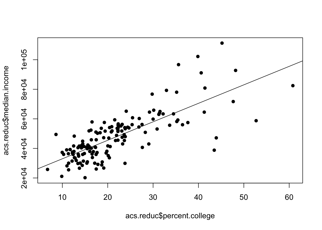
It looks pretty reasonable, but let’s reveal which points belong to what states.
plot(acs.reduc$percent.college[acs.reduc$state.abbr=="MS"], acs.reduc$median.income[acs.reduc$state.abbr=="MS"], col="firebrick", pch=16)
points(acs.reduc$percent.college[acs.reduc$state.abbr=="NY"], acs.reduc$median.income[acs.reduc$state.abbr=="NY"], col="darkblue", pch=16)
abline(m, col="black")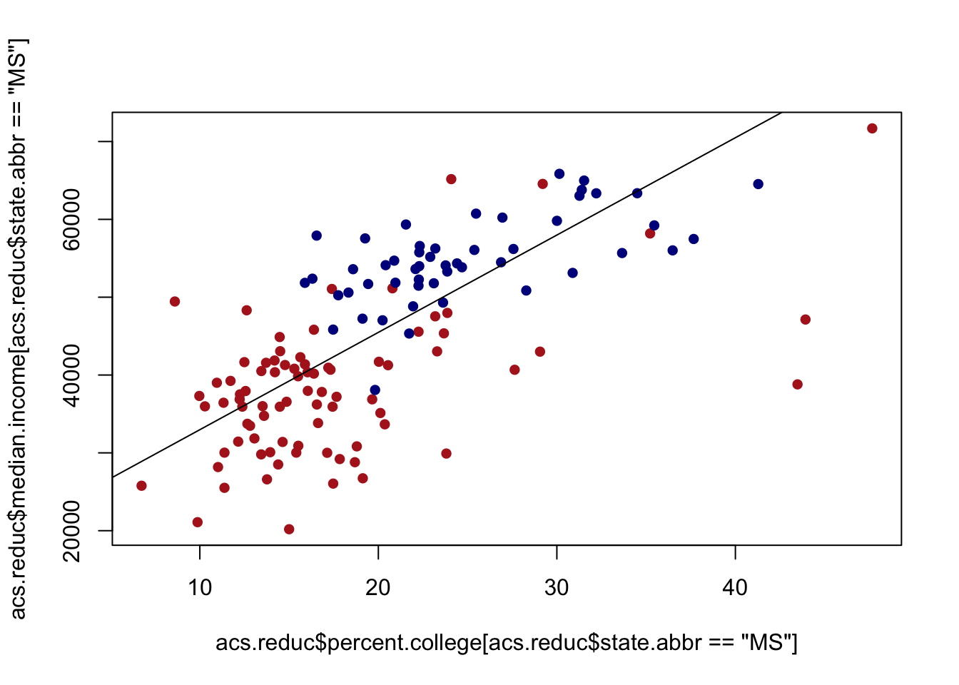
When we reveal that we start to see the problem of auto-correlation. The points for Mississippi are, on average, below the line. The points for New York are, on average, above the line. This means that for points within those clusters the errors are correlated.
Again, we can see this in a residual plot:
acs.reduc$resid <- residuals(m)

plot(acs.reduc$percent.college[acs.reduc$state.abbr=="MS"], acs.reduc$resid[acs.reduc$state.abbr=="MS"], col="firebrick", pch=16)
points(acs.reduc$percent.college[acs.reduc$state.abbr=="NY"], acs.reduc$resid[acs.reduc$state.abbr=="NY"], col="darkblue", pch=16)
abline(h=0)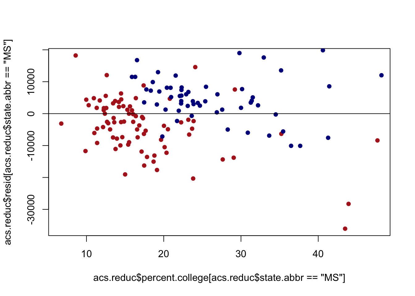
How do we fix this problem?
The first, and, simplest method is to simply use a method of calculating standard errors that takes into account the clustered structure of your data.
Above, we used the sandwhich package to generate heteroskedastic-robust standard errors. We can use the same package to generate clustered standard errors. In the vcovCL() function we can specify what variable our data are clustered on. Here it is state, so I’ve put that variable into the command. I’ve also included type="HC1" into this. This is actually the default so I didn’t have to put it in, but I wanted to point out that cluster standard errors are also heteroskedastic robust as well! A bonus!
m <- lm(median.income ~ percent.college, data=acs.reduc)
summary(m)
Call:
lm(formula = median.income ~ percent.college, data = acs.reduc)

Residuals:
   Min     1Q Median     3Q    Max
-36050  -6140   1073   5270  34248

Coefficients:
                Estimate Std. Error t value Pr(>|t|)
(Intercept)     20468.08    2133.36   9.594   <2e-16 ***
percent.college  1250.74      89.04  14.047   <2e-16 ***
---
Signif. codes:  0 '***' 0.001 '**' 0.01 '*' 0.05 '.' 0.1 ' ' 1

Residual standard error: 10380 on 142 degrees of freedom
Multiple R-squared:  0.5815,    Adjusted R-squared:  0.5786
F-statistic: 197.3 on 1 and 142 DF, p-value: < 2.2e-16library(sandwich)
cluster.vcov <- vcovCL(m, cluster= ~ state.abbr, type="HC1")
cluster.vcov2 <- vcovCL(m, cluster= ~ state.abbr)
#Compare to original var-covar matrix
vcov(m) (Intercept) percent.college
(Intercept) 4551246.2 -173642.147
percent.college -173642.1 7927.854#New hypothesis test
coeftest(m, vcov = cluster.vcov )
t test of coefficients:

                Estimate Std. Error t value  Pr(>|t|)
(Intercept)     20468.08    1048.71  19.517 < 2.2e-16 ***
percent.college  1250.74     154.34   8.104 2.223e-13 ***
---
Signif. codes:  0 '***' 0.001 '**' 0.01 '*' 0.05 '.' 0.1 ' ' 1
#You can also put the new variance covariance matrix into stargazer:
#Extract standard errors from new vcov matrix:
cluster.se <- sqrt(diag(cluster.vcov))
#(I just have to copy and paster that list(NULL) part of it as I always forget how to do it.)
stargazer(m, type="text", se=list(NULL,cluster.se))
===============================================
                        Dependent variable:
                    ---------------------------
                           median.income
-----------------------------------------------
percent.college            1,250.737***
                             (89.038)

Constant                   20,468.080***
                            (2,133.365)

-----------------------------------------------
Observations                    144
R2                             0.582
Adjusted R2                    0.579
Residual Std. Error    10,378.420 (df = 142)
F Statistic          197.322*** (df = 1; 142)
===============================================
Note:               *p<0.1; **p<0.05; ***p<0.01
While “fixing the standard errors” works in this situation, a more blatant problem here is that this simply isn’t a great model for what we are seeing in the data. To properly understand the relationship between schooling and income there are clearly a large numebr of confounding factors that can make counties in New York have both a large percentage of people with a college degree and a high median income.
A more fair comparison might simply be to look at the relationship within the two states.
We’ve already seen how to do this! We can use an indicator variable to set a different intercept for NY. (Here we just need the one because counties are either in NY or MS).
acs.reduc$ny <- acs.reduc$state.abbr=="NY"

m2<- lm(median.income ~ percent.college + ny, data=acs.reduc)
summary(m2)
Call:
lm(formula = median.income ~ percent.college + ny, data = acs.reduc)

Residuals:
   Min     1Q Median     3Q    Max
-24236  -5145   -412   3957  35078

Coefficients:
                Estimate Std. Error t value Pr(>|t|)
(Intercept)     22573.20    1863.06  12.116  < 2e-16 ***
percent.college   906.70      90.86   9.979  < 2e-16 ***
nyTRUE          12612.24    1782.45   7.076 6.39e-11 ***
---
Signif. codes:  0 '***' 0.001 '**' 0.01 '*' 0.05 '.' 0.1 ' ' 1

Residual standard error: 8947 on 141 degrees of freedom
Multiple R-squared:  0.6912,    Adjusted R-squared:  0.6868
F-statistic: 157.8 on 2 and 141 DF,  p-value: < 2.2e-16
The coefficient on nyTRUE indicates that the average median income in NY is around $12000 higher than in MS, holding constant the effect of education. If we use these numbers to graph this out:
plot(acs.reduc$percent.college[acs.reduc$state.abbr=="MS"], acs.reduc$median.income[acs.reduc$state.abbr=="MS"], col="firebrick", pch=16)
abline(a=coef(m2)["(Intercept)"], b=coef(m2)["percent.college"], col="firebrick")
points(acs.reduc$percent.college[acs.reduc$state.abbr=="NY"], acs.reduc$median.income[acs.reduc$state.abbr=="NY"], col="darkblue", pch=16)
abline(a=coef(m2)["(Intercept)"] + coef(m2)["nyTRUE"], b=coef(m2)["percent.college"], col="darkblue")
Let’s look at a residual plot of this graph:
acs.reduc$resid <- residuals(m2)

plot(acs.reduc$percent.college[acs.reduc$state.abbr=="MS"], acs.reduc$resid[acs.reduc$state.abbr=="MS"], col="firebrick", pch=16)
points(acs.reduc$percent.college[acs.reduc$state.abbr=="NY"], acs.reduc$resid[acs.reduc$state.abbr=="NY"], col="darkblue", pch=16)
abline(h=0)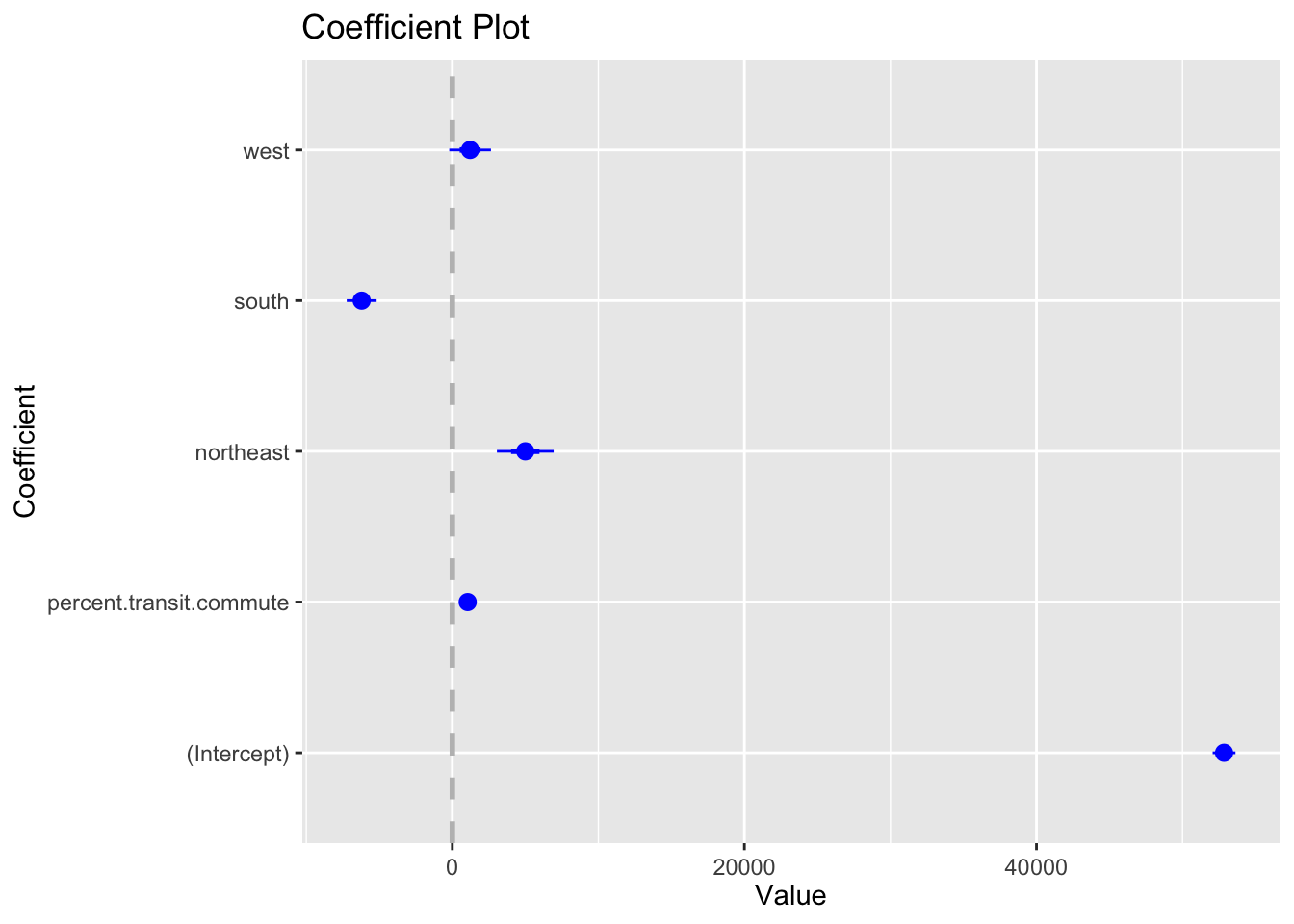
The residuals are now much more random! So an additional way of dealing with this auto-correlation is to model the data in a way that takes away that problem. There will be one caveat to this below, however.
We could imagine applying this same logic to this relationship to the entire dataset:
plot(acs$percent.college, acs$median.income, col="black", pch=16)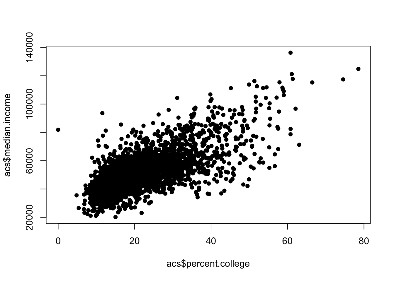
We might think the same problem exists in all the data. These are not a “random sample” but are actually observations from states, and there are unobserved things that will make the errors in CA correlate, and the erros in CT correlate, and the errors in DE correlate etc….
So in this case we may want to do something similar and fix our standard errors to account for this:
#Standard OLS
m <- lm(median.income ~ percent.college, data=acs)
summary(m)
Call:
lm(formula = median.income ~ percent.college, data = acs)

Residuals:
   Min     1Q Median     3Q    Max
-37849  -6044   -623   5696  52223

Coefficients:
                Estimate Std. Error t value Pr(>|t|)
(Intercept)     29651.55     435.98   68.01   <2e-16 ***
percent.college  1016.55      18.52   54.90   <2e-16 ***
---
Signif. codes:  0 '***' 0.001 '**' 0.01 '*' 0.05 '.' 0.1 ' ' 1

Residual standard error: 9789 on 3139 degrees of freedom
  (1 observation deleted due to missingness)
Multiple R-squared:  0.4899,    Adjusted R-squared:  0.4897
F-statistic:  3014 on 1 and 3139 DF,  p-value: < 2.2e-16
#Cluster standard errors
cluster.vcov <- vcovCL(m, cluster = ~ state.abbr)
coeftest(m, cluster.vcov)
t test of coefficients:

                 Estimate Std. Error t value  Pr(>|t|)
(Intercept)     29651.551   1337.982  22.161 < 2.2e-16 ***
percent.college  1016.547     55.331  18.372 < 2.2e-16 ***
---
Signif. codes:  0 '***' 0.001 '**' 0.01 '*' 0.05 '.' 0.1 ' ' 1
Or we could take the more extreme step and only look at the variation within states by including an indicators for each state. We can do that manually using a factor variable, but it’s going to be super unwieldy:
acs$state <- as.factor(acs$state.abbr)
m2 <- lm(median.income ~ percent.college + state, data=acs)
summary(m2)
Call:
lm(formula = median.income ~ percent.college + state, data = acs)

Residuals:
   Min     1Q Median     3Q    Max
-35915  -4858   -449   4544  47495

Coefficients:
                 Estimate Std. Error t value Pr(>|t|)
(Intercept)      46755.66    1655.59  28.241  < 2e-16 ***
percent.college    912.97      18.32  49.824  < 2e-16 ***
stateAL         -21096.75    1918.67 -10.996  < 2e-16 ***
stateAR         -20750.19    1889.23 -10.983  < 2e-16 ***
stateAZ         -17529.52    2742.22  -6.392 1.88e-10 ***
stateCA          -6873.33    1961.78  -3.504 0.000466 ***
stateCO         -19116.50    1935.97  -9.874  < 2e-16 ***
stateCT          -3381.02    3451.98  -0.979 0.327437
stateDC         -16710.50    8790.68  -1.901 0.057404 .
stateDE          -9369.81    5229.17  -1.792 0.073257 .
stateFL         -17783.53    1916.27  -9.280  < 2e-16 ***
stateGA         -18150.37    1742.94 -10.414  < 2e-16 ***
stateHI          -1214.25    4175.73  -0.291 0.771234
stateIA         -11435.15    1820.37  -6.282 3.82e-10 ***
stateID         -17750.20    2062.17  -8.608  < 2e-16 ***
stateIL         -11181.58    1814.49  -6.162 8.09e-10 ***
stateIN         -10598.85    1837.02  -5.770 8.73e-09 ***
stateKS         -16431.21    1808.40  -9.086  < 2e-16 ***
stateKY         -18396.02    1788.30 -10.287  < 2e-16 ***
stateLA         -18904.43    1932.92  -9.780  < 2e-16 ***
stateMA          -9705.59    2824.94  -3.436 0.000599 ***
stateMD          -1083.99    2384.50  -0.455 0.649429
stateME         -20002.21    2685.66  -7.448 1.22e-13 ***
stateMI         -16938.75    1859.65  -9.109  < 2e-16 ***
stateMN          -8668.97    1848.46  -4.690 2.85e-06 ***
stateMO         -17424.47    1793.33  -9.716  < 2e-16 ***
stateMS         -24291.55    1865.37 -13.022  < 2e-16 ***
stateMT         -19839.68    1972.35 -10.059  < 2e-16 ***
stateNC         -20201.99    1818.31 -11.110  < 2e-16 ***
stateND          -6023.26    1991.17  -3.025 0.002507 **
stateNE         -13895.60    1833.55  -7.579 4.59e-14 ***
stateNH          -9737.95    3166.90  -3.075 0.002124 **
stateNJ           -307.58    2482.49  -0.124 0.901404
stateNM         -23962.35    2210.37 -10.841  < 2e-16 ***
stateNV          -3712.33    2634.60  -1.409 0.158915
stateNY         -11745.19    1941.38  -6.050 1.62e-09 ***
stateOH         -11413.25    1846.57  -6.181 7.21e-10 ***
stateOK         -16927.43    1879.44  -9.007  < 2e-16 ***
stateOR         -17363.56    2151.04  -8.072 9.79e-16 ***
statePA         -12768.99    1916.17  -6.664 3.15e-11 ***
stateRI         -11403.91    4185.96  -2.724 0.006480 **
stateSC         -21428.18    2044.63 -10.480  < 2e-16 ***
stateSD         -15480.07    1920.55  -8.060 1.08e-15 ***
stateTN         -17363.67    1832.16  -9.477  < 2e-16 ***
stateTX         -12375.51    1691.58  -7.316 3.24e-13 ***
stateUT          -9294.74    2264.41  -4.105 4.15e-05 ***
stateVA         -12398.06    1767.81  -7.013 2.85e-12 ***
stateVT         -19288.06    2811.61  -6.860 8.28e-12 ***
stateWA         -13907.04    2114.63  -6.577 5.63e-11 ***
stateWI         -11671.03    1895.96  -6.156 8.44e-10 ***
stateWV         -18803.79    1982.07  -9.487  < 2e-16 ***
stateWY         -10009.15    2407.35  -4.158 3.30e-05 ***
---
Signif. codes:  0 '***' 0.001 '**' 0.01 '*' 0.05 '.' 0.1 ' ' 1

Residual standard error: 8621 on 3089 degrees of freedom
  (1 observation deleted due to missingness)
Multiple R-squared:  0.6107,    Adjusted R-squared:  0.6043
F-statistic: 95.01 on 51 and 3089 DF,  p-value: < 2.2e-16
Super hard to read!
Instead, we can recognize this as a broader “type” of regression; one where the data are clusters and we want to estimate our relationships within those clusters. To do so we use a “fixed effects” regression. A fixed effects regression is simply a regression where we include indicator variables for each of the clusters, less one. There are functions that will do this in a more straightforward way for us, however. There are actually a few packages that do this but I like felm() (“fixed-effects linear model”) from the lfe package
#install.packages("lfe")
library(lfe)
m.fe <- felm(median.income ~ percent.college | state.abbr, data=acs)
summary(m.fe)
Call:
   felm(formula = median.income ~ percent.college | state.abbr,      data = acs)

Residuals:
   Min     1Q Median     3Q    Max
-35915  -4858   -449   4544  47495

Coefficients:
                Estimate Std. Error t value Pr(>|t|)
percent.college   912.97      18.32   49.82   <2e-16 ***
---
Signif. codes:  0 '***' 0.001 '**' 0.01 '*' 0.05 '.' 0.1 ' ' 1

Residual standard error: 8621 on 3089 degrees of freedom
  (1 observation deleted due to missingness)
Multiple R-squared(full model): 0.6107   Adjusted R-squared: 0.6043
Multiple R-squared(proj model): 0.4456   Adjusted R-squared: 0.4364
F-statistic(full model):95.01 on 51 and 3089 DF, p-value: < 2.2e-16
F-statistic(proj model):  2482 on 1 and 3089 DF, p-value: < 2.2e-16
We can see this gives us exactly the same answer as the regression above, we just are supressing all of the dummy variables. We can see all them if we do:
getfe(m.fe) effect obs comp fe idx
state.abbr.AK 46755.66 29 1 state.abbr AK
state.abbr.AL 25658.91 67 1 state.abbr AL
state.abbr.AR 26005.47 75 1 state.abbr AR
state.abbr.AZ 29226.14 15 1 state.abbr AZ
state.abbr.CA 39882.33 58 1 state.abbr CA
state.abbr.CO 27639.16 64 1 state.abbr CO
state.abbr.CT 43374.63 8 1 state.abbr CT
state.abbr.DC 30045.16 1 1 state.abbr DC
state.abbr.DE 37385.85 3 1 state.abbr DE
state.abbr.FL 28972.12 67 1 state.abbr FL
state.abbr.GA 28605.29 159 1 state.abbr GA
state.abbr.HI 45541.41 5 1 state.abbr HI
state.abbr.IA 35320.51 99 1 state.abbr IA
state.abbr.ID 29005.46 44 1 state.abbr ID
state.abbr.IL 35574.08 102 1 state.abbr IL
state.abbr.IN 36156.81 92 1 state.abbr IN
state.abbr.KS 30324.44 105 1 state.abbr KS
state.abbr.KY 28359.63 120 1 state.abbr KY
state.abbr.LA 27851.23 64 1 state.abbr LA
state.abbr.MA 37050.07 14 1 state.abbr MA
state.abbr.MD 45671.66 24 1 state.abbr MD
state.abbr.ME 26753.44 16 1 state.abbr ME
state.abbr.MI 29816.90 83 1 state.abbr MI
state.abbr.MN 38086.68 87 1 state.abbr MN
state.abbr.MO 29331.18 115 1 state.abbr MO
state.abbr.MS 22464.10 82 1 state.abbr MS
state.abbr.MT 26915.97 56 1 state.abbr MT
state.abbr.NC 26553.67 100 1 state.abbr NC
state.abbr.ND 40732.40 53 1 state.abbr ND
state.abbr.NE 32860.05 93 1 state.abbr NE
state.abbr.NH 37017.70 10 1 state.abbr NH
state.abbr.NJ 46448.08 21 1 state.abbr NJ
state.abbr.NM 22793.31 32 1 state.abbr NM
state.abbr.NV 43043.32 17 1 state.abbr NV
state.abbr.NY 35010.46 62 1 state.abbr NY
state.abbr.OH 35342.41 88 1 state.abbr OH
state.abbr.OK 29828.23 77 1 state.abbr OK
state.abbr.OR 29392.09 36 1 state.abbr OR
state.abbr.PA 33986.67 67 1 state.abbr PA
state.abbr.RI 35351.75 5 1 state.abbr RI
state.abbr.SC 25327.48 46 1 state.abbr SC
state.abbr.SD 31275.59 66 1 state.abbr SD
state.abbr.TN 29391.99 95 1 state.abbr TN
state.abbr.TX 34380.15 254 1 state.abbr TX
state.abbr.UT 37460.91 29 1 state.abbr UT
state.abbr.VA 34357.59 133 1 state.abbr VA
state.abbr.VT 27467.59 14 1 state.abbr VT
state.abbr.WA 32848.61 39 1 state.abbr WA
state.abbr.WI 35084.62 72 1 state.abbr WI
state.abbr.WV 27951.87 55 1 state.abbr WV
state.abbr.WY 36746.51 23 1 state.abbr WYThe only complication to the idea of “hey, let’s just model the clusters and then the errors will be uncorrelated” is that best practices is to still use clustered standard errors in a fixed effect model. Why this is the case is actually beyond my stats ability, I just know that is best practice. The felm command actually makes this super simple, however. The command works as felm(model | fixed effect variable | instrumental variable| cluster variable, data). We won’t be using instrumental variables here, so we can just enter that as 0:
m.fe.cl <- felm(median.income ~ percent.college | state.abbr | 0 | state.abbr, data=acs)
summary(m.fe.cl)
Call:
   felm(formula = median.income ~ percent.college | state.abbr |      0 | state.abbr, data = acs)

Residuals:
   Min     1Q Median     3Q    Max
-35915  -4858   -449   4544  47495

Coefficients:
                Estimate Cluster s.e. t value Pr(>|t|)
percent.college   912.97        47.85   19.08   <2e-16 ***
---
Signif. codes:  0 '***' 0.001 '**' 0.01 '*' 0.05 '.' 0.1 ' ' 1

Residual standard error: 8621 on 3089 degrees of freedom
  (1 observation deleted due to missingness)
Multiple R-squared(full model): 0.6107   Adjusted R-squared: 0.6043
Multiple R-squared(proj model): 0.4456   Adjusted R-squared: 0.4364
F-statistic(full model, *iid*):95.01 on 51 and 3089 DF, p-value: < 2.2e-16
F-statistic(proj model):   364 on 1 and 50 DF, p-value: < 2.2e-16
#Much higher standard error!Assumption 2 is the “functional form” assumption, which says that your data was generated by the model that you have specified. The two violations of this are generally: non-linear relationships and interactions.
Let me give an example:
library(AER)
data("CASchools")
head(CASchools)
district school county grades students teachers
1 75119 Sunol Glen Unified Alameda KK-08 195 10.90
2 61499 Manzanita Elementary Butte KK-08 240 11.15
3 61549 Thermalito Union Elementary Butte KK-08 1550 82.90
4 61457 Golden Feather Union Elementary Butte KK-08 243 14.00
5 61523 Palermo Union Elementary Butte KK-08 1335 71.50
6 62042 Burrel Union Elementary Fresno KK-08 137 6.40
calworks lunch computer expenditure income english read math
1 0.5102 2.0408 67 6384.911 22.690001 0.000000 691.6 690.0
2 15.4167 47.9167 101 5099.381 9.824000 4.583333 660.5 661.9
3 55.0323 76.3226 169 5501.955 8.978000 30.000002 636.3 650.9
4 36.4754 77.0492 85 7101.831 8.978000 0.000000 651.9 643.5
5 33.1086 78.4270 171 5235.988 9.080333 13.857677 641.8 639.9
6 12.3188 86.9565 25 5580.147 10.415000 12.408759 605.7 605.4#Creating Variables
CASchools$STR <- CASchools$students/CASchools$teachers
summary(CASchools$STR) Min. 1st Qu. Median Mean 3rd Qu. Max.
14.00 18.58 19.72 19.64 20.87 25.80 CASchools$score <- (CASchools$read + CASchools$math)/2
summary(CASchools$score) Min. 1st Qu. Median Mean 3rd Qu. Max.
605.6 640.0 654.5 654.2 666.7 706.8 #Changing names
dat <- CASchools
library(ggplot2)
p <- ggplot(dat, aes(x=income, y=score)) + geom_point() +
labs(x="Avereage Household Income", y = "School Test Scores") +
geom_smooth(method = lm, formula = y ~ poly(x, 1), se = FALSE)
p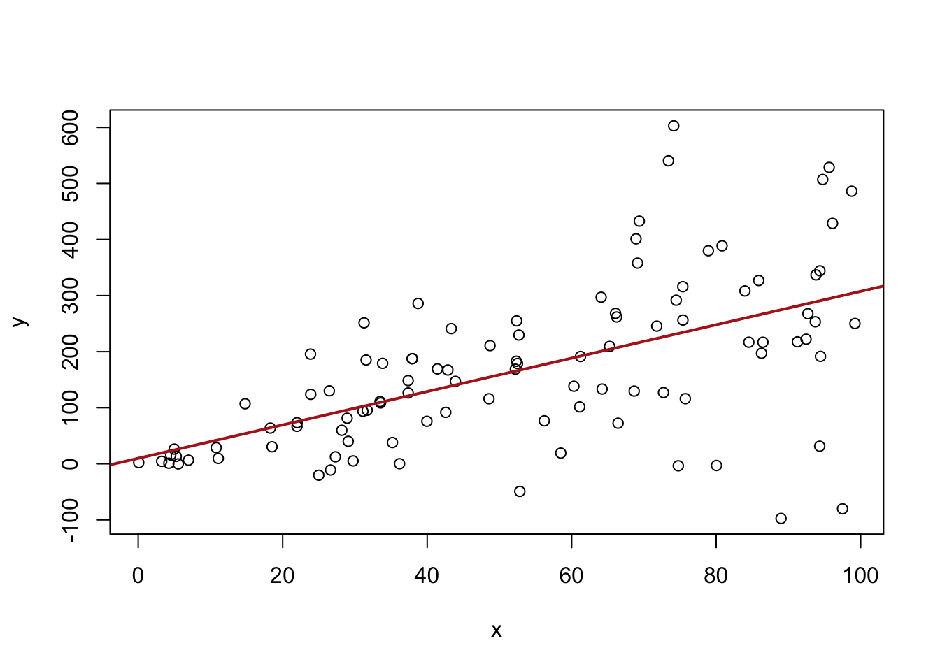
summary(lm(score ~ income, data=dat))
Call:
lm(formula = score ~ income, data = dat)

Residuals:
    Min      1Q  Median      3Q     Max
-39.574  -8.803   0.603   9.032  32.530

Coefficients:
            Estimate Std. Error t value Pr(>|t|)
(Intercept) 625.3836     1.5324  408.11   <2e-16 ***
income        1.8785     0.0905   20.76   <2e-16 ***
---
Signif. codes:  0 '***' 0.001 '**' 0.01 '*' 0.05 '.' 0.1 ' ' 1

Residual standard error: 13.39 on 418 degrees of freedom
Multiple R-squared:  0.5076,    Adjusted R-squared:  0.5064
F-statistic: 430.8 on 1 and 418 DF,  p-value: < 2.2e-16
Just looking at this visually, does this line well represent this relationship? Not really, no.
If I was to describe this relationship, I would say that test scores improve a lot when household income goes from 5 to 25, and then the effect levels off
The way we deal with this is adding polynomial terms to our regression. The easy way to think about polynomials is: it let’s the line curve.
A slightly better way to think about it is: we want to the relationship between income and test scores to change across the levels of income. When income is low the relationship is more steep, when income is high the relationship is more shallow
To do this we modify the simple bivariate regression by adding an additional variable income squared:
\[ \begin{aligned} y = a + bx + e\\ y = a + b_1 x + b_2 x^2 + e \end{aligned} \]
To implement this we can use the poly() function:
#YOU MUST USE THE RAW=T OPTION WHEN YOU USE THE POLY FUNCTION
#OR IT WILL NOT WORK

m <- lm(score ~ poly(income, 2, raw=T), data=dat )
summary(m)
Call:
lm(formula = score ~ poly(income, 2, raw = T), data = dat)

Residuals:
    Min      1Q  Median      3Q     Max
-44.416  -9.048   0.440   8.347  31.639

Coefficients:
                           Estimate Std. Error t value Pr(>|t|)
(Intercept)               607.30174    3.04622 199.362  < 2e-16 ***
poly(income, 2, raw = T)1   3.85099    0.30426  12.657  < 2e-16 ***
poly(income, 2, raw = T)2  -0.04231    0.00626  -6.758 4.71e-11 ***
---
Signif. codes:  0 '***' 0.001 '**' 0.01 '*' 0.05 '.' 0.1 ' ' 1

Residual standard error: 12.72 on 417 degrees of freedom
Multiple R-squared:  0.5562,    Adjusted R-squared:  0.554
F-statistic: 261.3 on 2 and 417 DF,  p-value: < 2.2e-16
#This is equivalent to:
dat$income2 <- dat$income^2
m <- lm(score ~ income + income2, data=dat )
summary(m)
Call:
lm(formula = score ~ income + income2, data = dat)

Residuals:
    Min      1Q  Median      3Q     Max
-44.416  -9.048   0.440   8.347  31.639

Coefficients:
             Estimate Std. Error t value Pr(>|t|)
(Intercept) 607.30174    3.04622 199.362  < 2e-16 ***
income        3.85099    0.30426  12.657  < 2e-16 ***
income2      -0.04231    0.00626  -6.758 4.71e-11 ***
---
Signif. codes:  0 '***' 0.001 '**' 0.01 '*' 0.05 '.' 0.1 ' ' 1

Residual standard error: 12.72 on 417 degrees of freedom
Multiple R-squared:  0.5562,    Adjusted R-squared:  0.554
F-statistic: 261.3 on 2 and 417 DF,  p-value: < 2.2e-16
#Plotting this relationship:
library(ggplot2)
p <- ggplot(dat, aes(x=income, y=score)) + geom_point() +
labs(x="Avereage Household Income", y = "School Test Scores") +
geom_smooth(method = lm, formula = y ~ poly(x, 2), se = FALSE)
p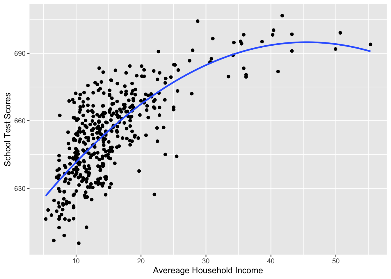
Visually fits much better.
Why does this work, and how can we describe the effect of x on y?
It’s now more complicated because the effect of income depends on what value of income we are talking about. As in, the steepness of the line varies across the level of income.
The tool that we use to calculate the slope of a line is a partial derivative from calculus.
In particular we are going to use the power rule, which states that:
\[ \begin{aligned} \frac{\partial y}{\partial x}(X^k) =k*X^{k-1} \\ \frac{\partial y}{\partial x}(aX^k) =k*aX^{k-1} \\ \frac{\partial y}{\partial x}(a) =0 \\ \frac{\partial y}{\partial x}(Z) =0 \end{aligned} \]
How does this apply to our standard regression equation?
\[ \begin{aligned} \hat{y} = \hat{\alpha} + \hat{\beta}*x + \hat{\beta}*Z \\ \frac{\partial y}{\partial x} = 1*\beta*x^0\\ \frac{\partial y}{\partial x} = \beta \end{aligned} \]
Which makes a lot of sense!
What is the effect of x when we add a polynomial term?
\[ \begin{aligned} \hat{y} = \hat{\alpha} + \hat{\beta_1}*x + \hat{\beta_2}*x^2 \\ \frac{\partial y}{\partial x} = \hat{\beta}_1 + 2*\hat{\beta_2}*x \end{aligned} \]
So here, if we wanted to know the effect of income when income is at 20
coef(m) (Intercept) income income2
607.30174351 3.85099392 -0.04230845 coef(m)[2] + 2*coef(m)[3]*20 income
2.158656 #2.15
#and at 30
coef(m)[2] + 2*coef(m)[3]*30 income
1.312487 #and at 50
coef(m)[2] + 2*coef(m)[3]*50 income
-0.3798508 The effect of x changes as x itself increases.
We could continue to add polynomial terms:
#Plotting this relationship:
library(ggplot2)
p <- ggplot(dat, aes(x=income, y=score)) + geom_point() +
  labs(x="Avereage Household Income", y = "School Test Scores") +
  geom_smooth(method = lm, formula = y ~ poly(x, 4), se = FALSE)
p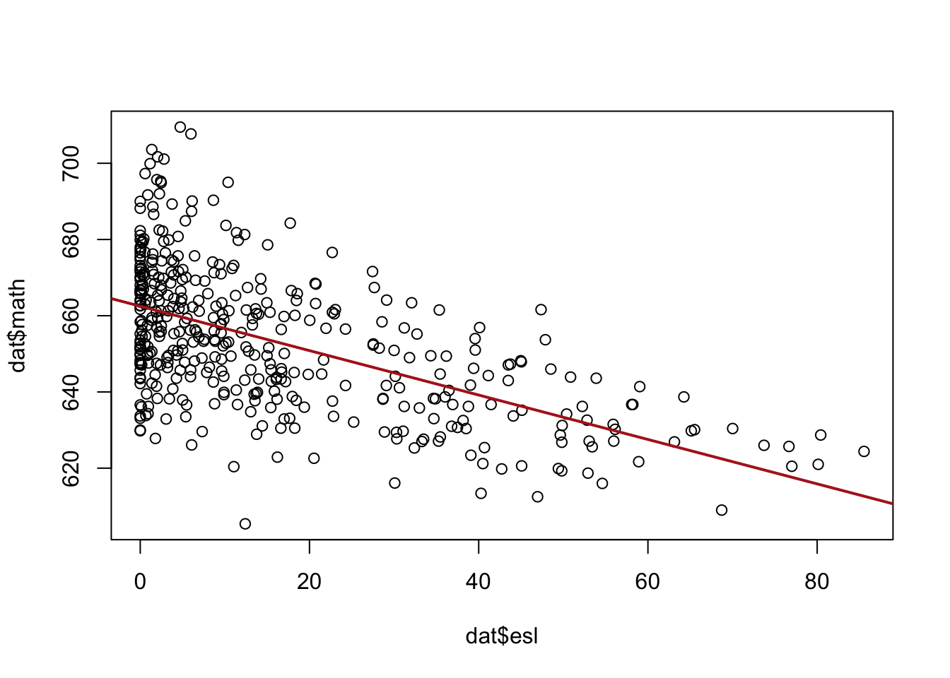
And we could use differentiations to determine the slope of that line:
\[ \begin{aligned} \hat{y} = \alpha + \beta_1*x + \beta_2*x^2 + \beta_3 * x^3 + \beta_4 *x^4\\ \frac{\partial y}{\partial x} = \beta_1 + 2*\beta_2*x + 3*\beta_3*x^2 + 4*\beta_4*x^3 \end{aligned} \]
At all these points:
m <- lm(score ~ poly(income, 4, raw=T), data=dat )
coef(m)
(Intercept) poly(income, 4, raw = T)1 poly(income, 4, raw = T)2
5.773402e+02 9.876232e+00 -4.342116e-01
poly(income, 4, raw = T)3 poly(income, 4, raw = T)4
9.791736e-03 -8.159040e-05 #20
coef(m)[2] + 2*coef(m)[3]*20 + 3*coef(m)[4]*20^2 + 4*coef(m)[5]*20^3poly(income, 4, raw = T)1
1.646959 #and at 30
coef(m)[2] + 2*coef(m)[3]*30 + 3*coef(m)[4]*30^2 + 4*coef(m)[5]*30^3poly(income, 4, raw = T)1
1.44946 #and at 50
coef(m)[2] + 2*coef(m)[3]*50 + 3*coef(m)[4]*50^2 + 4*coef(m)[5]*50^3poly(income, 4, raw = T)1
-0.9021091 Isn’t this better? Aren’t we getting a more exact fit? The \(r^2\) is almost certainly higher! That’s good, right?
Why might we not like doing this? Let’s remember the overall goal of describing the population-level data generating process. We think this is one of many samples of data. At the extreme we could fly around and capture every single bit of random variation in these data, but we don’t think that this is a good way to summarize what this relationship is in a way that might be generalizable to other samples of data. In the parlance of regression, we have to balance describing a plausible functional form for the data with not over-fitting our regression to this specific dataset. I would say the 4th-order polynomial is absolutely over-fitting.