coin <- c(0,1)3 Probability
📄 Download the R code from this chapter
📝 Download the class handout for this chapter
Pretty much all classes and textbooks that teach statistics start with some introductory material on probability theory. They get in the weeds of dice, card games, lotteries, colored balls in hats in a way that thoroughly confuses the students. There is then some hand-waving over the course of a week and then… ta-dah! P-values! If I’m to be honest, it was years before I was able to properly articulate the connection between probability theory and day-to-day statistics. It is indeed helpful to learn a bit of probability theory in order to understand the foundation of inferential statistics, but I promise here not to get too bogged down in weird probability exercises.
One resource that helped me enormously in seeing the connection between probability and statistics was the book “The Drunkard’s Walk” by Leonard Mlodinow. It’s a very entertaining read in the style of Malcolm Gladwell or Michael Lewis that tells the story of how statistics was founded. Here is an excerpt that is a good starting point:
Bill Miller was the sole portfolio manager of Legg Mason Value Trust Fund, who in each year of his fifteen-year streak beat the portfolio of equity securities that constitute Standard & Poor’s 500. For his accomplishments, Miller was heralded “the Greatest Money Manager of the 1990s” by Money magazine. In the fourteenth year of Miller’s streak, one analyst put the odds of a fourteen-year streak by chance alone at 372,529:1. Those who quoted the low odds were right in one sense: if you had singled out Bill Miller in particular at the start of 1991 in particular and calculated the odds that by pure chance the specific person you selected would beat the market for precisely the next fifteen years then those odds would indeed have been astronimcally low. But those are not the relevant odds because there are thousands of mutual fund managers (over 6000 currently) and there are many fifteen year periods in which the feat could have been accomplished. So the relevant question is, if thousands of people are tossing coins once a year and have been doing so for decades, what are the chances that one of them, for some peiod of fifteen years or longer, will toss all heads?
Mlodinow is providing an example of the “Hot Hand Fallacy”, which is the mistaken belief that streaks are less likely than they really are. This fallacy is very common in sports, for example, where coaches, analysts, and fans all assume a run of success (or failure!) for a player is meaningful, when in reality such streaks are quite common.
The question at hand here is whether what this particular investor has done is special, or not. We understand that there is a lot of randomness in the stock market, yet it is tempting to believe that there are individuals who can out-smart it and continuously win. The existence of a streak of winning this long must be nearly impossible to achieve only due to chance, right?
This question, which we’ll answer together via simulation below, helps clarify why probability is an important component of statistical inference. When trying to decide whether to be impressed by not by Bill Miller, our baseline is the question: if success and failure on the stock market was just random chance, how likely would it be that we see someone have 15 years of success? If it’s very likely to happen by random chance then we should not be impressed when we observe it happening in the real world!
In order for us to calculate this, we first need a way to calculate what is likely to happen due to chance variation alone. In other words, we need to be able to calculate the probability of random events.
We are not learning probability just to solve puzzles about coin streaks. Everything in the rest of this course rests on the notion that the summary statistics we compute from a sample (a mean, a proportion, a regression coefficient, whatever) are themselves random variables, which are processes with known features that generate data probabilistically.
Here is what that means. Say we run a poll of 8,000 Americans and find that 52% support Fetterman. That 52% is our estimate. But if we had polled a different 8,000 people, we would have gotten a slightly different number – maybe 51%, maybe 53%. That variation is not measurement error or noise. It is the value of a random variable whose distribution has knowable, calculable, properties. Our observed 52% is one draw from that random variable. And the entire job of statistics is to try to understand the predictable and regular features of that random variable well enough to say something disciplined about the truth we can never observe directly.
Getting to that understanding takes machinery we build across the next several chapters. Probability (this chapter) is the language for talking about randomness. Then random variables (the next two chapters) give us mathematical objects that let us describe data generating processes and compute their properties. Then sampling theory (a couple chapters after that) tells us the crucial result: when we compute a statistic from a sample, that statistic is itself a random variable with a knowable distribution. Once we have all that, we can do actual statistical inference – hypothesis tests, confidence intervals, the standard errors on regression coefficients, all of it.
But this chapter starts us off: how do we calculate the probability of a random event? Once we can do that, we start building the rest of the machinery.
3.1 The Basics of Probability
It is odd to define something that we use all the time in everyday language, but it’s helpful to lay out some clear definitions of what we mean by probability.
What do we mean, for example, when we say that a coin comes up heads 50% of the time? Or that a dice1 comes up as “4” \(\frac{1}{6}\) of the time?
We clearly do not mean that, for example, a coin must come up tails after coming up heads. Barring magic, each flip of the coin is independent from the last. Probability has nothing to say about what must happen on any particular coin flip.
Instead, what probability denotes is the expected long-term frequency of events. A definition that I find helpful:
The chance of something gives the percentage of time it is expected to happen, when the basic process is done over and over again, independently and under the same conditions.
This is a particularly helpful frame because, as we’ll see below, a good way for us to estimate probability is to simply to get R to repeat a process a whole bunch of times to determine the percentage of time an event is likely to happen.
To formalize our look into probability, two key terms are events and a sample space. Events are simply outcomes of a particular thing: the outcome of the roll of a dice or a flip of a coin; or the outcome of a presidential election; or whether a randomly sampled individual is favorable towards the President or not. A sample space is set of all possible outcomes of the thing we are considering. So for the roll of a dice the sample space is all of the numbers \(\lbrace 1,2,3,4,5,6 \rbrace\). For a flip of a coin \(\lbrace H,T \rbrace\). For the outcome of a presidential election \(\lbrace Dem, Rep, Third \rbrace\). For whether an individual is favorable towards the President \(\lbrace Fav, Unfav, No.Opinion \rbrace\).
When the probability of all events are equal (which of the above are equal?) we can then define the probability of an event occuring by dividing the number of elements in the event by the total number of events in the sample space.
So the probability of getting a heads on a coin flip is \(P(H) = \frac{1}{2}\). The probability of rolling a 2 is \(P(2) = \frac{1}{6}\).
This helpfully scales up when we are interested in multiple events ocurring. For example what is the probability of rolling an even number? \(P(even) = \frac{3}{6} = \frac{1}{2}\)
This method does not apply to when the probability of events ocurring is not equal. For example we cannot calculate the probability of a third party candidate winning an election by \(P(third) \neq \frac{1}{3}\).
There are a couple of “rules” (axioms) about probability that are helpful to keep in mind.
- The probability of any event A is non-negative:
\[ P(A)\geq 0 \]
An event can’t have a less than 0 probability of occurring.
- The probability that one of the outcomes in the sample space occurs is 1.
\[ P(\Omega) = 1 \]
The probability that something happens is a certainty, or 1.
Together these two axioms also tell us that probability ranges between 0 and 1 (or 0% and 100%, if we want to express it like that).
- If events A and B are mutually exclusive:
\[ P(AorB) = P(A) + P(B). \]
What do we mean by mutually exclusive? Simply that A occurring precludes B from occurring, and vice-versa. We can ask, for example, what is the probability of rolling a 2 or a 3? If you roll a 2 you can’t roll a 3; if you roll a 3 you can’t roll a 2.
So here:
\[ P(2or3) = P(2) + P(3) = \frac{1}{6} + \frac{1}{6} = \frac{1}{3} \]
We could confirm this visually by looking at the sample space
\[ \lbrace 1,\mathbf{2},\mathbf{3},4,5,6\rbrace. \]
But what if we ask a different question: what is the probability of rolling a 4 or an even number? Are these events mutually exclusive? No! If you roll an even number it doesn’t preclude rolling a 4.
Just looking visually if we think about the events in the sample space that satisfy this statement we see that the probability of this combined event is
\[ \frac{1}{2}: \lbrace 1,\mathbf{2},3,\mathbf{4},5,\mathbf{6}\rbrace. \]
But if we (incorrectly) apply Axiom 3 we get
\[ P(4orEven) \neq P(4) + P(Even) = \frac{1}{6} + \frac{1}{2} = \frac{4}{6}. \]
Because of this we use a more general formula for Axiom 3:
\[ P(AorB) = P(A) + P(B) - P(A\&B) \]
Notice what the last part of this equation is doing. We need to subtract off the probability of the events that are contained in both A & B so we don’t double count. In the example above the probability of rolling a 4 and rolling an even number is \(\frac{1}{6}\). So using this formula we get:
\[ P(4orEven) = P(4) + P(Even) - P(4\&Even) = \frac{1}{6} + \frac{1}{2} - \frac{1}{6}= \frac{1}{2} \]
Helpfully, this more general formula also applies to events that are mutually exclusive, because the probability of both of them occurring is 0!
The other helpful bit of notation is to think about the complement of an event, which is simply everything in the sample space that is not that event.
For example what is the complement of rolling a 2(\(2^c\))?
\[ \lbrace 1,3,4,5,6 \rbrace. \]
What is the complement of rolling an odd number (\(odd^c\))?
\[ \lbrace 2,4,6 \rbrace \]
This is helpful for the following reason: What is \(P(2 \text{ or } 2^c)\)? Using the formula from above:
\[ P(2 \text{ or } 2^c) = P(2) + P(2^c) - P(2\&2^c) = \frac{1}{6} + \frac{5}{6} - 0 = 1 \]
An event either happens or doesn’t happen, so any event plus its complement by definition equals 1.
So if we generalize that \(P(A) + P(A^c)=1\), then re-arranging we get:
\[ \begin{aligned} P(A) &= 1- P(A^c)\\ \text{and}&\\ P(A^c) &= 1- P(A) \end{aligned} \]
The probability of an event occurring is 1 minus the probability of that event not occurring. This ends up being very helpful!
3.1.1 Simulating Probability in R
There are ways of calculating probability mathematically that we will get to, but one of the beautiful things about learning statistics in the computer age is the ability to obtain estimates of probability via simulation. Instead of calculating what happens when you throw a dice an infinite number of times, we can just simulate the throwing of a dice a large number of times to get a proximate answer. Throughout this class we will continuously do things via “math” (old school calculations) and prove that we are right via “simulation” (using R to do something a large number of times).
The way that we do that using R is a for() loop.
We already saw this functionality in the R review chapter, and we will review it here.
Let’s say we want to know the odds of getting 0 heads when we flip a coin 7 times. There is a way to calculate this mathematically, but remember the probability of an event can be defined as the frequency that event occurs over the long run. We can get at this in R by literally flipping 7 coins a large number of times and seeing how often we get 0 heads.
Before we do this a large number of times, let’s create the code to do it once.
First, let’s create an object called coin that is just a vector with 0 and 1 in it. We’ll define 0 as tails, and 1 as heads.
The sample() command take a random sample from an object a specific number of times. Here we are going to sample from our object “coin” 7 times with replacement. The 7 times represents 7 flips of the coin. We are sampling with replacement here because each time you flip a coin you can get either heads or tails. It’s not the case that once you get a heads you can only get a tails.
Running this once we get the following output. As we’ve defined tails as 0 and heads as 1,
sample(coin,7,replace=T)[1] 0 1 1 0 0 1 1Sample() is a random command, however, so each time we run it we’ll get something different.
sample(coin,7,replace=T)[1] 0 1 1 1 1 1 1sample(coin,7,replace=T)[1] 0 0 0 1 1 1 1sample(coin,7,replace=T)[1] 1 0 1 1 1 1 0Finally, we aren’t interested in the specific sequence of heads and tails but just the number of heads each time we flip a coin 7 times. Because we’ve defined heads as the number 1 and tails as 0, taking the sum of the sample will give us the number of heads.
sum(sample(coin,7,replace=T))[1] 5Now we need to repeat this a large number of times. Let’s do 100000! A loop lets us repeat this same code as many times as we want. We’ll set up our loop just as we did above, going from 1 to 100,000. We can put our coin flipping code in the loop and see what happens.
for(i in 1:100000){
  sum(sample(coin,7,replace=T))
}
One nuance of running loops in R is that by default R will run the code in the background and not display anything. So in this case R did sample 7 coins 100,000 times, but because we didn’t save it anywhere there is no record of this. We need to explicitly save what is happening. We’ll create an empty vector “num.heads” to save these, and then each time through the loop save the outcome in each successive position in num.heads.
set.seed(19104)
num.heads <- rep(NA, 100000)
for(i in 1:100000){
 num.heads[i] <-  sum(sample(coin,7,replace=T))
}
head(num.heads)
[1] 3 3 3 2 2 4Finally, using the table command we can see exactly how often each of these outcomes happened. Around 780 out of the 100,000 times did none of the coins come up heads. Less than 1% of the time.
table(num.heads)num.heads
0 1 2 3 4 5 6 7
787 5551 16051 27450 27651 16201 5540 769 prop.table(table(num.heads))num.heads
0 1 2 3 4 5 6 7
0.00787 0.05551 0.16051 0.27450 0.27651 0.16201 0.05540 0.00769 Now let’s simulate the throwing of a dice in R. First, how might we set it up so we throw a dice once? I am going to create an object called “dice” that is a vector containing the possible outcomes of a dice throw. I’m then going to use the sample() function to randomly sample 1 number from this vector. The beginning of the code uses set.seed see the footnote for what this is.2
set.seed(19104)
dice <- c(1,2,3,4,5,6)
sample(dice,1,replace=T)
[1] 4Here the random sampling produced a dice roll of 4.
Let’s go further to roll this dice a large number of times in a way that approximates the probability of getting each number, 1 through 6. I create a loop that is 10,000 iterations. In each iteration I sample from our object dice and save the output in the empty vector result. At the end of the loop the vector result will be 10,000 items long, with each being the result of a single dice throw.
set.seed(19104)
dice <- c(1,2,3,4,5,6)
result <- rep(NA,10000)
  for(i in 1:10000){
    result[i] <- sample(dice,1,replace=T)
  }
table(result)
result
1 2 3 4 5 6
1684 1653 1710 1682 1676 1595 We know that each number of a fair dice will come up 1/6 of the time, so our expectation would be that each of these numbers would be drawn \(10000/6=1666\) times. Obviously with random chance we don’t get that number exactly, but each is quite close.
3.1.2 Permutations & Combinations
It’s pretty easy to talk about the probability with one coin or easy things like that, which might have you thinking we are over-complicating something that is very straightforward. Where probability is more helpful is sharpening our thinking for more complex events.
Consider the following problem. I have a locker in Pottruck and I’m worried about someone trying to guess the code to my locker. The lock on my locker has 50 numbers and my code (and any code) has three unique numbers that need to be put in the right order. What is the probability that someone guesses my combination?
Using the probability we have learned so far, we can break this problem down in the following way. Each event is a possible combination. There is only 1 correct event, so we need to know the probability of selecting the 1 right answer out of all the possible answers. In other words:
\[ P(GuessRight) = \frac{1}{AllPermutations} \]
Now I’ve used “Permutation” instead “Combination” here on purpose. In probability theory a permutation is a sequence where the order matters (as it does when putting in a locker code), where “combination” is a sequence that doesn’t matter (like a lottery drawing).
So how many different 3-digit permutations are there to a lock with 50 numbers? We can break it down like this: There are 50 possibilities for the first number in the code. Because the numbers have to be unique, there are 49 digits for the second number. Finally, because the first two numbers can’t be repeated, there are 48 possibilities for the last number. In total the number of permutations is: \(50*49*48=117600\).
Therefore the probability of guessing my code is \(\frac{1}{117600}\).
As above, we can similarly use R to get an answer to this question:
#Estimating the probability of guessing a locker combination

#Set Seed
set.seed(19104)

#Draw prime combination
prime <- sample(seq(1,50),3, replace=F)

#How do we determine if two vectors are exactly equal?
c(2,34,29)==prime
[1] FALSE FALSE FALSE#Use the all command to determine if all numbers match
all(c(28,21,37)==prime)[1] TRUE#Use a loop to repeatedly sample and check
results <- rep(NA, 1E6)
for(i in 1:length(results)){
results[i] <- all(sample(seq(1,50),3, replace=F)==prime)
}
prop.table(table(results))results
FALSE TRUE
0.99999 0.00001 #Approximately equivalent to what we calculated via math. There is a more generalized formula to determine the number of permutations which is:
\[_nP_k = \frac{n!}{(n-k)!}\]
which gives the number of permutatations where \(n\) is the number of options and \(k\) is the number of selections. Plugging the numbers from above into this:
\[ \begin{aligned} _{50}P_3 &= \frac{50!}{(50-3)!} \\ &= \frac{50 \cdot 49 \cdot 48 \cdot 47 \cdot 46 \dots \cdot 2 \cdot 1}{47 \cdot 46 \dots \cdot 2 \cdot 1}\\ &= 50 \cdot 49 \cdot 48 = 117{,}600 \end{aligned} \]
A combination differs from a permutation because with a combination the order does not matter. A lottery is a great example of this. You win the lottery if the numbers you selected come out of the bin, regardless of the order of the balls.
Let’s try to calculate the probability of winning the Mega Millions lottery. For this lottery you have to match 5 white balls that are drawn from a pool of 70, as well as one gold “MegaBall” drawn from a pool of 25. To win the jackpot you need the exact winning combination so the probability of winning is: \(\frac{1}{\#Of Possiblg Combos}\).
Let’s deal first with the white balls. Using the permutations formula (which is wrong) we would get:
\[_nP_k = \frac{70!}{(70-5)!} \approx 1.5bil\]
But that’s the number of permutations such that two sequences with the same numbers in a different order would be treated as different lottery drawings. So to get the number of combinations do we have to increase or decrease this number?
Decrease! If any sequence of the same numbers is treated as equal, we collapse all of those into 1. So to get the number of combinations we have to divide by the number of ways to sequence a series of 5 numbers. The ways to sequnece 5 numbers is \(5!\). So to generalize, the formula for combinations just modifies the permutations formula to be:
\[_nC_k = \frac{n!}{k!(n-k)!}\]
Therefore the number of combinations for the 5 white balls is:
\[_{70}C_5 =\frac{70!}{5!(70-5)!} = 12103014\]
A lot less!
To get this number I used R. There is a very helpful function for combinations:
choose(70,5)[1] 12103014To get the total odds of winning the lottery we also have to deal with the gold ball. The way to think about that is that for every possible sequence of white numbers there are 25 possibilities for the gold ball. So the total number of possible lottery numbers are: \(12103014*25 = 302575350\).
Here’s a problem for us to solve: When is it a good idea to play the lottery?
We can think of the expected value of the lottery (or anything) as being equal to the benefits minus the costs:
\[ E[Lottery] = p(win)*Prize - Cost \]
The cost of the lottery is 2 dollars, so the lottery starts to become a good thing to do when \(p(win)*Prize\) becomes equal to 2:
We can solve this via algebra, solving for \(P\), the prize, given what we know about the odds and the cost:
\[ \begin{aligned} \frac{1}{302575350}*P &=&2\\ P&=&2*302575350 \\ P &=& 605150700 \end{aligned} \]
The expected value of playing Mega Millions is equal to the $2 cost when the jackpot is just over 600 million. Which it is frequently! Should you therefore play the lottery every time the value gets over this number? No. You shouldn’t, because we are ignoring a critical and unknown component to the lottery. Can you guess what it is? 3
Another common probability problem we can solve with permutations is the “Birthday problem”. What is the probability in a classroom of 20 people that two people will have the same birthday? To solve this it is helpful to use what we learned above about complements. It turns out re-framing this question makes things a bit easier: what is the probability that nobody shares a birthday in a class?
The sample space we are interested in here is all possible permutations of 20 birthdays. Each “event” is a sequence of 20 birthdays. The probability we want to calculate is
\[ P(No Shared Birthdays) = \frac{\text{Number of sequences with no shared birthdays}}{\text{All possible sequences of birthdays}} \]
Let’s start with the denominator: What is the size of the entire sample space? Here we are interested in every possible set of 20 birthdays, including the ones with repeats. So if we take the first person in a class of 20 there are 365 possible birthdays for them to have. Because we are not interested in unique birthdays for the denominator, the second person also has 365 options for a birthday. And so on. So to get the total number of sequences 20 people can have birthdays on we get \(365*365*365*365 \dots\), or \(365^{20}\). Note that this calculation gives the total number of sequences where order matters.
For the numerator, we need to find the number of sequences where there is no repeating birthdays. In other words, how many ways are there to uniquely order 20 birthdays when there are 365 possible birthdays. This is just like the locker permutation but scaled up. We get:
\[ _{365}P_{20} = \frac{365!}{(365-20)!} \]
You might think it’s odd we are calculating a permutation (order matters) rather than a combination (order doesn’t matter) here. Why are we treating (October 1, January 2) different from (January 2, October 1) in determining the number of birthday combinations? This is because we calculated the denominator as \(365^20\), which is all possible sequence of birthdays where order matters. If we wanted we could have divided that number by \(20!\) to make order not matter, but that would mean we are just dividing the numerator and denominator by the same number, and we we would get the same result.
So to calculate the probability of no-two people sharing a birthday in a class of 20 we will calculate:
\[ \frac{\frac{365!}{(365-20)!}}{365^{20}} \]
OK, let’s try to do that:
num <- factorial(365)/factorial(345)
num
[1] NaNWe get nothing! What! Why?? Because \(365!\) is an absolutely gigantic number that R literally cannot calculate.
In order to calculate this we can make use of the choose() function in R which we used above. Because this calculates a combination, however, it is calculating: \(\frac{365!}{20!(365-20)!}\). To get the permutations we multiply the whole thing by \(20!\).
(choose(365,20)*factorial(20))/365^20[1] 0.5885616So the probability of nobody in a class of 20 people sharing a birthday is only 58.9 percent. Using our knowledge of complements, this means the probability that two people (or more) share a birthday in a class of 20 people is 41%! That’s very high.
Again, we can make our lives less mathy by simulating the birthday problem in R:
First, how can we randomly assign birthdays to 20 people using R? We can think of this in the same way as above. We can create a vector birthdays that is numbered 1 to 365 to represent all the possible days of the year (sorry, leap day babies). We can then sample from that vector 20 possibilities, with replacement. anyDuplicated() returns a 0 if there are no duplicates in a vector, and returns the index position of the first duplicate if there is one. So, if this returns a number greater than 0, there is a duplicate in the sampled vector.
set.seed(19104)
birthdays <- seq(1,365,1)
s <- sample(birthdays, 20, replace=T)
s
[1] 156 277 119 101 334 276 86 279 178 225 305 329 212 195 5 261 365 335 192
[20] 24anyDuplicated(s)>0[1] FALSEIn this first run of the simulation, all 20 students have a unique birthday.
Now, again, let’s run this a large number of times to estimate the probability of people sharing a birthday:
set.seed(19104)
birthdays <- seq(1,365,1)
result <- rep(NA, 10000)
for(i in 1:10000){
  s <- sample(birthdays, 20, replace=T)
  result[i] <- anyDuplicated(s)>0
}
table(result)
result
FALSE TRUE
5891 4109 In these 10,000 runs, over 41% of them had duplicated birthdays – The exact same as we calculated with math!
Can we make a graph that is the probability of at least two people sharing a birthday for every class size from 5 to 100? Can we make it both using math and simulation?
set.seed(19104)
birthdays <- seq(1,365,1)
class.size <- seq(5,100,1)
prob.sim <- rep(NA, length(class.size))
prob.math <- rep(NA, length(class.size))

for(j in 1:length(class.size)){
result <- rep(NA, 10000)
for(i in 1:10000){
  s <- sample(birthdays, class.size[j], replace=T)
  result[i] <- anyDuplicated(s)>0
}
prob.sim[j] <- mean(result)
prob.math[j] <- 1-(choose(365,class.size[j])*factorial(class.size[j]))/365^class.size[j]
}

plot(class.size, prob.math, col="dodgerblue", type="b", xlab="Class Size",
     ylab="Probability of Shared Birthday", pch=16)
points(class.size, prob.sim, col="firebrick", type="b", pch=16)
legend("topleft", c("Math","Simulation"), pch=c(1,1), col=c("dodgerblue", "firebrick"))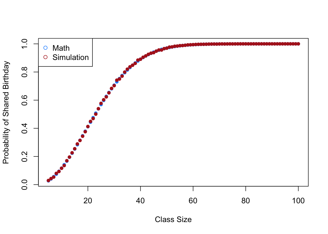
Some more practice writing loops to simulate probability (see end of chapter for answers).
Rolling 4 dice, and we want to know the odds of the dice all coming up as the same number.
Rolling two dice, what are the odds of the sum of the two dice equaling 10?
Rolling two dice, what are the odds of each sum, 2 to 12? Plot the result.
Bag 1 containes 3 red and 5 black balls. Bag 2 contains 4 red and 4 black balls. A bag is chosen at random, and then a ball is chosen at random from that bag. What’s the probability a red ball is drawn?
The Philadelphia Phillies are expected to beat the Washington Nationals 60% of the time. In a stretch of 7 games, what are the odds that the Phillies win a majority (4 games)?
Estimate the probability the Phillies win the majority of 9,11,13,15…61 games, and plot the result.
3.2 Conditional probability
An additional complication with probability is to think about conditional probability: how the probability of an event changes based on what else we already know.
Consider rolling two dice. Because each die is independent and has 6 possible outcomes, the full sample space has \(6 \times 6 = 36\) outcomes, and (crucially) they are all equally likely. We can write it out as a grid, where each cell shows the sum of the two dice:
| 1 | 2 | 3 | 4 | 5 | 6 | |
|---|---|---|---|---|---|---|
| 1 | 2 | 3 | 4 | 5 | 6 | 7 |
| 2 | 3 | 4 | 5 | 6 | 7 | 8 |
| 3 | 4 | 5 | 6 | 7 | 8 | 9 |
| 4 | 5 | 6 | 7 | 8 | 9 | 10 |
| 5 | 6 | 7 | 8 | 9 | 10 | 11 |
| 6 | 7 | 8 | 9 | 10 | 11 | 12 |
Because these 36 outcomes are equally likely, we can compute the probability of any event by just counting the cells where it happens and dividing by 36. So, for example, what is the probability the sum is at least 8?
Highlighting the cells where the sum is \(\geq 8\):
| 1 | 2 | 3 | 4 | 5 | 6 | |
|---|---|---|---|---|---|---|
| 1 | 2 | 3 | 4 | 5 | 6 | 7 |
| 2 | 3 | 4 | 5 | 6 | 7 | 8 |
| 3 | 4 | 5 | 6 | 7 | 8 | 9 |
| 4 | 5 | 6 | 7 | 8 | 9 | 10 |
| 5 | 6 | 7 | 8 | 9 | 10 | 11 |
| 6 | 7 | 8 | 9 | 10 | 11 | 12 |
We can count 15 bold cells, so:
\[ P(\text{sum} \geq 8) = \frac{15}{36} = \frac{5}{12} \]
Now consider a related but different question: suppose I tell you the first die came up 5. What is the probability the sum is at least 8?
The key insight to conditional probability is that this is a subsetting question. Once we know the first die is 5, we are no longer working with the full 36-outcome sample space. We are working with just the 6 outcomes in the row where die 1 = 5:
| 1 | 2 | 3 | 4 | 5 | 6 | |
|---|---|---|---|---|---|---|
| 5 | 6 | 7 | 8 | 9 | 10 | 11 |
Within this restricted sample space, four of the six outcomes have sum \(\geq 8\). So:
\[ P(\text{sum} \geq 8 \mid \text{die 1} = 5) = \frac{4}{6} = \frac{2}{3} \]
Knowing that the first die was 5 raised the probability of the sum being \(\geq 8\) from about 42% to about 67%. That’s what “conditioning” does: it changes the sample space we are working with, which changes the probability.
Every conditional probability is a subsetting operation. Restrict to the outcomes consistent with the condition, then count within that restricted set.
The more general formula:
\[ P(A \mid B) = \frac{P(A \& B)}{P(B)} \]
We can verify this on our example.
- \(P(\text{sum} \geq 8 \text{ AND die 1} = 5) = \frac{4}{36}\) (the four bold cells in the die 1 = 5 row)
- \(P(\text{die 1} = 5) = \frac{6}{36}\) (the six cells in that row)
\[ P(\text{sum} \geq 8 \mid \text{die 1} = 5) = \frac{4/36}{6/36} = \frac{4}{6} = \frac{2}{3} \checkmark \]
Why does dividing by \(P(B)\) work? Because “restrict to a smaller sample space” is exactly what dividing by the total probability mass of that smaller space does mathematically. Once we know \(B\) happened, all outcomes outside \(B\) have probability zero and we need the remaining probabilities to re-scale so they still sum to 1.
As a gut check, does \(P(A \mid B) = P(B \mid A)\)?
No! These are completely different, almost unrelated, questions. We just computed:
\[ P(\text{sum} \geq 8 \mid \text{die 1} = 5) = \frac{2}{3} \]
For \(P(\text{die 1} = 5 \mid \text{sum} \geq 8)\), we restrict to the 15 cells where the sum is \(\geq 8\) (the bold cells across the whole grid), and count how many have die 1 = 5. That is (5,3), (5,4), (5,5), (5,6) — 4 cells.
\[ P(\text{die 1} = 5 \mid \text{sum} \geq 8) = \frac{4}{15} \approx 0.27 \]
Very different from \(\frac{2}{3}\)! The question matters. “Given the first die was 5, what’s the probability the sum is \(\geq 8\)?” is a completely different question than “Given the sum is \(\geq 8\), what’s the probability the first die was 5?”
3.2.1 Independence
Now that we have the concept of conditional probability in our pockets it allows us to formally define the concept of “independent” events.
Simply: two events A&B are independent when the probability of A does not change when B takes on different values.
Formally:
\[ \begin{aligned} P(A|B) &= P(A)\\ \text{and}&\\ P(B|A) &= P(B) \end{aligned} \]
To give a (purposely) absurd example, consider rolling a dice and flipping a coin. What is the probability of rolling a 2 conditional on flipping a head?
The full sample space has 12 equally likely outcomes:
| Tails | Heads |
|---|---|
| T1 | H1 |
| T2 | H2 |
| T3 | H3 |
| T4 | H4 |
| T5 | H5 |
| T6 | H6 |
So to test for independence we can determine if \(P(2 \mid H) = P(2)\).
Compute \(P(2 \mid H)\): use the conditional probability formula. The outcome \(H \& 2\) is a single cell (H2), and there are 6 outcomes with heads.
\[ P(2 \mid H) = \frac{P(H \& 2)}{P(H)} = \frac{1/12}{6/12} = \frac{1}{6} \]
Compute \(P(2)\): two outcomes have die = 2 (T2 and H2) out of 12.
\[ P(2) = \frac{2}{12} = \frac{1}{6} \]
Both are \(\frac{1}{6}\), so \(P(2 \mid H) = P(2)\) and the two events are independent. Which makes sense — knowing the coin came up heads shouldn’t tell you anything about what the die rolled.
3.2.2 The Monty Hall Problem
Perhaps the most famous of all conditional probability problems is the “Monty Hall” problem. This was a real TV show that even I’m not old enough to have actually seen. Here’s the setup to the problem:
You are on a game show and must choose one of three doors, where one conceals a new car and two conceal goats. After you randomly choose one door, the host of the game show, Monty, opens a different door, which does not conceal a car. Then, Monty asks you if you would like to switch to the unopened third door. You will win the new car if it is behind the door of your final choice. Should you switch, or stay with your original choice?
After reading this prompt, most people implicitly think of the sample space being something like this:
| Stay | Switch |
|---|---|
| Car → Car | Car → Goat1 |
| Goat1 → Goat1 | Car → Goat2 |
| Goat2 → Goat2 | Goat1 → Car |
| Goat1 → Goat2 | |
| Goat2 → Car | |
| Goat2 → Goat1 |
Now, as we will see this sample space is wrong for some reasons that are usually omitted in the telling of the Monty Hall problem. But if we assumed this was true, what is \(P(Car|Stay)\) and \(P(Car|Switch)\)?
In this (wrong) version of the sample space, both of these are \(1/3\). In one of three scenarios when you stay you win the car (the scenario where you randomly pick right on your first selection). In 2 of the 6 scenarios when you switch you win the car: when you initially pick one of the goats and then you switch to the door with the car.
The reason the Monty Hall problem trips people up is that the sample space actually looks like this:
| Stay | Switch |
|---|---|
| Car → Car | Car → Goat1 or Goat2 |
| Goat1 → Goat1 | Goat1 → Car |
| Goat2 → Goat2 | Goat2 → Car |
Note that the top row of the switch column combines what look like two outcomes (Monty could open either goat door) into one, because both leave you with a goat. From your perspective, ending up with Goat 1 and ending up with Goat 2 are the same result.
If you are in the “switch” condition, only three things can actually happen.
First, you can initially select the Car. In this case, Monty will randomly decide to open the door containing either Goat 1 or Goat 2, and you will switch to the other Goat. It doesn’t actually matter which Goat you are switching to. If you initially select the car (with 1/3 probability), switching will always get you a Goat.
If you initially select a Goat (either 1 or 2), Monty will reveal the other goat. The only door left to switch to is the one with the car.
To make this clear, look at the two rows that disappeared from our table: Goat2 → Goat1 & Goat1 → Goat2. What would have to happen for this sequence to occur? You would initially select a door with a goat. Monty would then open the door with the car. You would then switch to the other door (which you know definitely does not have a car). Indeed: Monty will always reveal a door with a goat behind it. He will never reveal the door with the car behind it.
Because of these things when we recalculate the conditional probabilities: \(P(Car|Stay)=1/3\) and \(P(Car|Switch) = 2/3\). We can count rows directly here because each of the three real switch scenarios is equally likely. Each corresponds to one of your three possible initial door picks, and each initial pick has probability 1/3.
The most helpful way for me to think about it is this: What is the probability of winning a car conditional on picking a goat first and switching? \(P(Car|Goat_1 \& Switch) = 1\). You are certain to win a car if you pick a goat first and switch. Because \(P(Goat)=2/3\) that is also the probability of winning if you always switch.
That may or may not make sense, but we can also prove this works by doing it in R.
Here is a simple simulation of the Monty Hall problem where the player picks either a goat with 2/3 probability and a car with 1/3 probability, and then either switches or stays:
This simulation also introduces if() statements within R loops. As you will see below an if() statement allows us to run a certain code block only if a condition is met. This is helpful because what the player gets from switching changes based on whether they picked a car or a goat first.
#First I will write one game without a loop:

#Pick a door, which unbeknownst to us contains a goat or a car:
pick <- sample(c("goat","goat","car"),1)

#If the player stays they get their initial selection
stay = pick

#If they switch, what happens depends on what their initial pick is

if(pick=="car"){
  #If they initially picked car, switching necessarily gets them a goat.
  switch = "goat"
} else {
  #If they initially picked a goat, switching necessarily gets them the car.
  #This is the key to the whole thing. Monty never reveals the car, so if you pick
  #a goat he *must* reveal the other goat.
  switch="car"
}
stay
[1] "goat"switch[1] "car"#Now put this whole thing in a loop, capturing what happens if you stay vs switch for
#each initial selection:
stay <- NA
switch <- NA
for(i in 1:10000){
pick <- sample(c("goat","goat","car"),1)
stay[i] = pick
if(pick=="car"){
switch[i] = "goat"
} else {
switch[i]="car"
}
}
mean(stay=="car")[1] 0.3369mean(switch=="car")[1] 0.6631I’ve also written a slightly more complicated simulation of the MH problem that more explicitly captured each step and Monty’s decision making. Each of the 10,000 times we will (1) randomly assign the car to a door, (2) have the player randomly choose a door, (3) Have Monty semi-randomly open a door, (4) record whether the car is won if the player stays, and if the car is won if they player switches.
#One Monty Hall game
set.seed(19104)
#Randomply place the Cars and goats
placement <- sample(c("Goat", "Goat","Car"),3, replace=F)
#In this case the placement is Goat, Goat, Car

#Person randomly selects a door:
door.selection <- sample(seq(1,3),1)
#In this case the person has selected door 1, that has a goat

#Now Monty must open a door
#He can't open the door we have opened, and can't open the door with the car
#Record which doors have goats:
goats <- which(placement=="Goat")
#Can't open the door you've selected
goats <- goats[goats!=door.selection]
#We are going to use an if statement here to represent the two situations
#In this situation there is only one door Monty can open, but if we had chosen the car first
#there would be two doors that monty can open and he has to choose one
if(length(goats)==1){
  open <- goats
} else {
  open <- sample(goats,size=1)
}
#
#The door that is switched to is the remaining door
switch.selection <- c(1,2,3)[c(-door.selection,-open)]

#Finally we see if the car is won either in the stay or switch condition
#Stay
placement[door.selection]=="Car"
[1] FALSE#Switch
placement[switch.selection]=="Car"[1] TRUE#In this case the car is won when switching.
#It should be clear from this that if you pick a goat initially and switch you *necessarily* win
#the car. Because you have a 2/3 probability of picking a goat, you win the car 2/3 of the time if you
#switch. Is that what R says?
win.stay <- rep(NA, 1000)
win.switch <- rep(NA, 1000)
for(i in 1:1000){
#Placement
placement <- sample(c("Goat", "Goat","Car"),3, replace=F)
#Person randomly selects a door:
door.selection <- sample(seq(1,3),1)
#Now Monty must open a door
goats <- which(placement=="Goat")
goats <- goats[goats!=door.selection]
if(length(goats)==1){
open <- goats
} else {
open <- sample(goats,size=1)
}
switch.selection <- c(1,2,3)[c(-door.selection,-open)]
win.stay[i] <- placement[door.selection]=="Car"
win.switch[i] <- placement[switch.selection]=="Car"
}
table(win.stay)win.stay
FALSE TRUE
670 330 table(win.switch)win.switch
FALSE TRUE
330 670 3.3 Calculating the odds of Stock Market Predictions
Let’s return to the motivating example of this chapter: financial adviser Bill Miller. Remember that Miller had an “unprecedented” streak of 15 straight years of success in beating the S&P 500. Is this an interesting or impressive thing to happen?
How can we go about examining this? The way probability (and eventually, statistics) focuses our minds is to have us answer the following question: If an investor’s ability to beat the S&P 500 is truly random (50% Success, 50% failure), how likely is it that an investor will have a streak of 15 consecutive years of success? If what we observe is very likely to happen via random chance then it is a less impressive thing to have happen. Put the other way: if what we observe is very unlikely to happen by random chance then it is impressive!
There are ways to calculate this mathematically, but R allows us to get at these answers in a different way: through simulation. If our baseline model is that success and failure is 50/50, then we can think about it as flipping a coin. As we saw above, with R we don’t have to calculate what happens when we flip a coin a bunch of times, we can just flip a coin a bunch of times.
Above, Mlodinow pointed out that some pundits calculated the odds of this happening as being extremely low, but this calculation was wrong.
Let’s first calculate this the wrong way. Here’s what we want to simulate for this wrong way: if we flip a coin 15 times, how often do we get all heads? This represents the situation where a particular investor, over a particular period of time, has all successes.
Here is the code that simulates this in R:
set.seed(19104)
coin <- c(0,1)

all.heads <- rep(NA, 1000000)

for(i in 1:length(all.heads)){
  s <- sample(coin, 15, replace=T)
  all.heads[i] <- sum(s)==15
}

sum(all.heads)
[1] 33To review our ability to simulate, here breakdown of what is happening in this code:
The first command is
set.seed(19104): this command makes it so R’s random number generator will start in the same place each time we run this code. The following is still a “random” process, this command just makes it so we have the same “random” process each time this code is run. Otherwise we’d get a slightly different answer each time.I then create an object that will function as a coin, which is just a vector of 0 (tails) and 1 (heads).
This code flips a coin 15 times, one million times. That is, imagine a flipping a coin 15 times: this is doing this process once. We then flip that coin 15 times, 999,999 more times.
all.heads <- rep(NA,1000000)creates an empty vector 1 million spaces long to store the results of the simulation.We then begin a loop that runs one million times.
s <- sample(coin, 15, replace=T)takes a sample of the coin object that is 15 units long, and saves it to an objects.Finally,
all.heads[i] <- sum(s)==15evaluates whether in this sample all the flips are heads (True) or not (False).
We see that the output of this simulation above is that in 33/1000000 simulations does the coin come up all heads. So if this is the question we are asking, it is indeed very special for that to happen.
What Mlodinow is pointing out, however, is that this is the wrong question to be asking. Miller was not the only financial adviser working during this period (there are thousands), and a streak doesn’t have to happen in the exact 15 year period for which it happened to Miller.
So we need to re-frame the question. If 6000 financial advisers are picking stocks for 40 years, what are the odds that any of them have a 15 year run of success? Put into the terms of a coin: if 6000 people are all flipping a coin once a year for 40 years, what are the odds that any of them get a streak of 15 heads in a row during that time period?
Let’s use our R skills to answer that question.
First, let’s simulate 6000 financial advisers picking stocks randomly for 40 years. In terms of coin flip chances: if 6000 people are all flipping a coin each year for 40 years, do any of them get 15 heads in a row?
One person flipping a coin 40 times looks like:
set.seed(19104)
coin <- c(0,1)
s <- sample(coin, 40, replace=T)
s
[1] 1 0 1 0 0 0 1 1 0 0 1 0 1 0 0 0 0 1 0 1 1 1 0 0 0 0 0 1 1 1 0 0 0 0 0 1 1 0
[39] 0 0The function rle gives the length of streaks in the data, but keep in mind we are only interested in streaks of 1s.
rle(s)$lengths [1] 1 1 1 3 2 2 1 1 1 4 1 1 3 5 3 5 2 3rle(s)$values [1] 1 0 1 0 1 0 1 0 1 0 1 0 1 0 1 0 1 0rle(s)$lengths[rle(s)$values==1][1] 1 1 2 1 1 1 3 3 2sort(rle(s)$lengths[rle(s)$values==1], decreasing = T)[1] 3 3 2 2 1 1 1 1 1There are two streaks of 5, one streak of 4 etc. Because we have sorted this column the longest streak will be the first entry. So we just need to see if that is at least 15.
sort(rle(s)$lengths[rle(s)$values==1], decreasing = T)[1]>=15[1] FALSENow that’s one adviser flipping a coin for 40 years. But there are 6000 advisers. Let’s iterate this over 6000 advisers, storing for each whether they had a streak over 15:
str.res <- NA
for(i in 1:6000){
  s <- sample(coin, 40, replace=T)
  str.res[i] <- sort(rle(s)$lengths[rle(s)$values==1], decreasing = T)[1]>=15
}
table(str.res)
str.res
FALSE TRUE
5996 4 any(str.res)[1] TRUEIn this one instance, 4 advisers had a string of successes that was at least 15 long. But this is not probability yet: this is just one instance of 6000 advisers picking stocks randomly for 40 years. To turn this into probability we need to do this whole operation a large number of times.
First, let’s turn the above block into a function where we can input the number of advisers, the number of years, and the streak length, and it returns whether any of the advisers had a streak of the specified length.
adv.streak <- function(n.adv, n.yrs, streak){
  str.res <- NA
  for(i in 1:n.adv){
    s <- sample(coin, n.yrs, replace=T)
    str.res[i] <- sort(rle(s)$lengths[rle(s)$values==1], decreasing = T)[1]>=streak
  }
  return(any(str.res))
}
So to simulate, again, 6000 advisors over 40 years and seeing if any have a streak of 15 successes:
adv.streak(n.adv=6000, n.yrs = 40, streak=15)[1] TRUEAnd now let’s simulate that whole thing 100 times to see the probability that someone would get a lucky string of 15 wins if all advisers were doing was picking randomly:
any.lucky <- NA
for(i in 1:100){
any.lucky[i] <- adv.streak(n.adv=6000, n.yrs = 40, streak=15)
}
table(any.lucky)
any.lucky
FALSE TRUE
6 94 In 94 of the 100 simulations did at least one financial adviser have a run of 15 successful years in a row. So contra Money magazine, it would be incredibly weird if someone didn’t have a run of 15 successes in a row!
Now that we have made a function we can answer similar questions with different paramaters.
Maybe I am the owner of a small boutique trading firm with 5 employees. One of them has beat the s&p all 10 years we’ve been open. What’s the odds of that?
any.lucky <- NA
for(i in 1:1000){
any.lucky[i] <- adv.streak(n.adv=5, n.yrs = 10, streak=10)
}
table(any.lucky)
any.lucky
FALSE TRUE
988 7 Only about 2.2% of the time would one of my 5 traders achieve this by luck alone. This seems like I might actually have a special employee.
3.4 Coming Next
What we have built in this chapter is the machinery for computing the probability of specific events: rolling a certain number, flipping a certain sequence, or seeing a certain streak. Next chapter we take a step up in abstraction. Instead of computing “the probability of 15 heads in a row,” we describe the underlying randmoness as a data generating process called a random variable. Random variables allow us to define parameters (expected value, variance) that we can use to summarize an entire DGP without having to simulate every possible outcome. It is a big step toward where we are headed: sampling and inference.
3.5 Problem Answers
- Rolling 4 dice, and we want to know the odds of the dice all coming up as the same number.
set.seed(19104)
dice <- c(1,2,3,4,5,6)
result <- rep(NA, 10000)
for(i in 1:10000){
  s <- sample(dice,4, replace=T)
  result[i] <- var(s)==0
}

mean(result)
[1] 0.0051- Rolling two dice, what are the odds of the sum of the two dice equaling 10?
set.seed(19104)
dice <- c(1,2,3,4,5,6)

result <- rep(NA, 10000)

for(i in 1:10000){
  roll <- sample(dice,2, replace=T)
  result[i] <- sum(roll)==10
}

mean(result)
[1] 0.0835- Rolling two dice, what are the odds of each sum, 2 to 12? Plot the result.
set.seed(19104)
dice <- c(1,2,3,4,5,6)

result <- rep(NA, 10000)

for(i in 1:10000){
 roll <- sample(dice,2, replace=T)
result[i] <- sum(roll)
}

table(result)
result
2 3 4 5 6 7 8 9 10 11 12
290 549 837 1122 1419 1648 1377 1122 835 531 270 barplot(prop.table(table(result)),
xlab="Sum of Two Dice",
ylab="P(Sum)")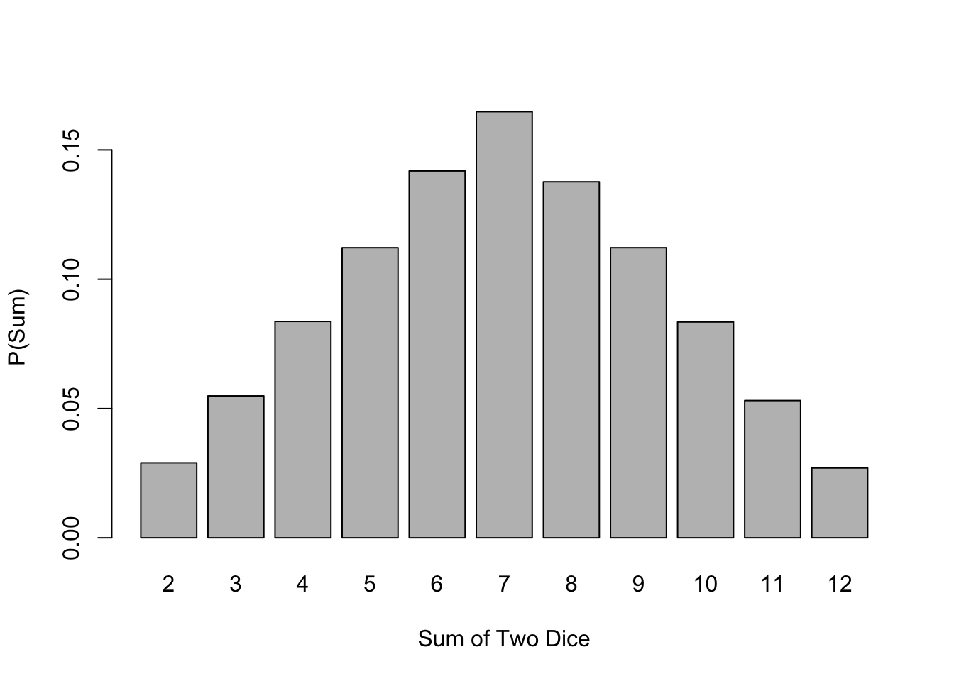
- Bag 1 containes 3 red and 5 black balls. Bag 2 contains 4 red and 4 black balls. A bag is chosen at random, and then a ball is chosen at random from that bag. What’s the probability a red ball is drawn?
set.seed(19104)
bag1 <- c(rep("R",3), rep("B",5))
bag2 <- c(rep("R",4), rep("B",4))

bags <- cbind(bag1,bag2)

result <- rep(NA,10000)

for(i in 1:length(result)){
  bag <- sample(1:2,1)
  ball <- sample(bags[,bag], 1)
  result[i] <- ball=="R"
}

mean(result)
[1] 0.4343- The Philadelphia Phillies are expected to beat the Washington Nationals 60% of the time. In a stretch of 7 games, what are the odds that the Phillies win a majority (4 games)?
philly.truth <- c(rep(1,6), rep(0,4))
result <- rep(NA,10000)
for(i in 1:length(result)){
  result[i] <- mean(sample(philly.truth, 7, replace=T))>.5
}
mean(result)
[1] 0.7103- Estimate the probability the Phillies win the majority of 9,11,13,15…61 games, and plot the result.
philly.truth <- c(rep(1,6), rep(0,4))
series.length <- seq(7,61,2)
percent.series.win <- rep(NA, length(series.length))

for(j in 1:length(percent.series.win)){
 result <- rep(NA,10000)
 for(i in 1:length(result)){
   result[i] <- mean(sample(philly.truth, series.length[j], replace=T))>.5
 }
percent.series.win[j] <-  mean(result)
}

plot(series.length, percent.series.win, type="b", pch=16)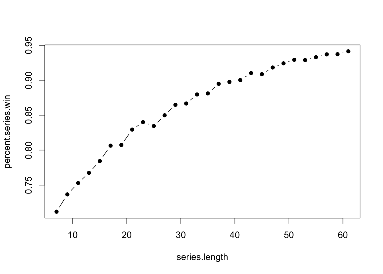
The Oxford English Dictionary now recognizes “dice” as both the plural and singular form. Language changes. Don’t @ me.↩︎
The short version of what this is: setting a seed before this code ensures that you get the same output everytime you run it. If I didn’t have this command in here I would get a different result everytime I ran
sample(dice,1,replace=T). Because I am writing notes and want the output to the same everytime I compile this code, I useset.seed()in these commands so that I (and you, if you’re running the code on your machine) get the exact same results. The slightly longer explanation is that R has many commands that give us a “random” output. But the output R gives is actually pseudo-random. If you start in the same place, the subsequent “randomly” generated outcomes will always be exactly the same. This is a feature, not a bug. It allows us to write code that produces random outcomes, but will also produce the same random outcomes if we run the code again. You can put whatever you want in the set.seed, but with the same input, anyone running R will get the same output. Throughout the course I use the Zip code of the University as the starting point for the Random Number Generator inside R.↩︎Human behavior. As the jackpot increases so does the number of people that decide to play. Each additional person playing the lottery means the odds of having to split the jackpot increase. As such the expected value of the lottery likely goes down at a certain point.↩︎