10 If & Functions
Updated for S2026? Yes.
One of the reasons it was helpful for you to learn For loops is because they have a lot of applicability in coding beyond just working in R. Two other operations that similarly have a lot of applicability are If statements and functions.
In short:
ifstatements allow us to choose certain bits of code that only run under a particular condition.Functions allow us generalize a specific bit of code whereby we give it certain inputs and it will produce certain outputs.
10.1 If statements
We have used conditional logic statements in multiple ways throughout this course. One thing that we have not done however, is use them to say: if a certain condition holds, run this code
We can do this via if statements. Similar to when we do this for a single line of code, we start with a logical statement – but in this case a statement that produces a single T or F, and then R will only run the code if the statement is True.
Here is some presidential election data:
pres <- rio::import("https://github.com/marctrussler/IDS-Data/raw/main/CountyPresData2020.Rds")
#> Warning: Missing `trust` will be set to FALSE by default
#> for RDS in 2.0.0.
This gives, for each county, the number of votes won by Biden, Trump, and other candidates in the 2020 presidential election.
What if we want, in each state, the winners margin? That is, how much did the winner of each state win by, in raw votes?
Because we want to do each state, we are going to need to use a loop.
As a start, let’s write a loop to calculate the total number of biden and trump votes in the state:
states <- unique(pres$state)
biden.votes <- rep(NA, length(states))
trump.votes <- rep(NA, length(states))

for(i in 1:length(states)){
  biden.votes[i] <- sum(pres$biden.votes[pres$state==states[i]])
  trump.votes[i] <- sum(pres$trump.votes[pres$state==states[i]])
}

head(cbind(states,biden.votes,trump.votes))
#>      states biden.votes trump.votes
#> [1,] "AK"   "153778"    "189951"
#> [2,] "AL"   "849624"    "1441170"
#> [3,] "AR"   "423932"    "760647"
#> [4,] "AZ"   "1672143"   "1661686"
#> [5,] "CA"   "11110250"  "6006429"
#> [6,] "CO"   "1804352"   "1364607"
That did we wanted to, but how can we write code within that loop to calcualte the winners margin?
The problem is that to calculate the winners margin we have to do something different if the winner is Biden or if the winner is Trump. So inside loop is we want to check, for the state we are currently working on, if biden.vote is greater than trump.vote. If it is, we want to calculate biden.votes - trump.votes. If it is not we want to calculate trump.votes-biden.votes.
Just to write out that logic we want to do:
states <- unique(pres$state)
biden.votes <- rep(NA, length(states))
trump.votes <- rep(NA, length(states))
winners.margin <- rep(NA, length(states))
for(i in 1:length(states)){
  biden.votes[i] <- sum(pres$biden.votes[pres$state==states[i]])
  trump.votes[i] <- sum(pres$trump.votes[pres$state==states[i]])

  #if biden votes is greater than trump votes
  winners.margin[i] <- biden.votes[i] - trump.votes[i]
  #Otherwise
  winners.margin[i] <- trump.votes[i] - biden.votes[i]
}

head(cbind(states,biden.votes,trump.votes))
To do this we have to use the if statement functionality.
If statements look a lot like for loops, but in the opening bracket we put a conditional statement that is either T or F. If the statement is T R will run what is in the squiggly brackets. If it is false it won’t:
if(2+2==4){
  print("I ran code chunk 1")
}
#> [1] "I ran code chunk 1"

if(2+2==5){
  print("I ran code chunk 2")
}
When we run the first bit of code it runs what is in the squiggly brackets, when we run the second chunk of code it does not run what is in the squiggly brackets.
Right now our code just says: if the statement is true run this code, if it is not, move on. But many times (and for the example we are returning to), we want to say: if this statement is true run this code, if it is not, run this other code. In that case we can add an else to our code:
if(2+2==5){
  print("I ran code chunk 2")
} else {
  print("I ran code chunk 3")
}
#> [1] "I ran code chunk 3"
Because the logical statement at the start is false, R runs the code following the else.
It’s worth thinking for a minute of why this doesn’t accomplish the same thing:
On first blush this does the same as the above, printing code chunk 3 when the logical statement is false. However, if the logical statement is true it will print both things, which is not what we want:
if(2+2==4){
  print("I ran code chunk 2")
}
#> [1] "I ran code chunk 2"
print("I ran code chunk 3")
#> [1] "I ran code chunk 3"
We aren’t limited to just two conditions, we can use else if to add a second logical statement:
if(2+2==5){
  print("I ran code chunk 1")
} else if(2+2==4){
  print("I ran code chunk 2")
} else {
  print("I ran code chunk 3")
}
#> [1] "I ran code chunk 2"
But if we change second statement:
if(2+2==5){
  print("I ran code chunk 1")
} else if(2+2==6){
  print("I ran code chunk 2")
} else {
  print("I ran code chunk 3")
}
#> [1] "I ran code chunk 3"
Let’s use this to edit our example of calculating the winners margin in each state:
states <- unique(pres$state)
biden.votes <- rep(NA, length(states))
trump.votes <- rep(NA, length(states))
winners.margin <- rep(NA, length(states))
for(i in 1:length(states)){
  biden.votes[i] <- sum(pres$biden.votes[pres$state==states[i]])
  trump.votes[i] <- sum(pres$trump.votes[pres$state==states[i]])

  if(biden.votes[i] >trump.votes[i]){
    winners.margin[i] <- biden.votes[i] - trump.votes[i]
  } else {
    winners.margin[i] <- trump.votes[i] - biden.votes[i]
  }
}
cbind(states, winners.margin)
#>       states winners.margin
#>  [1,] "AK"   "36173"
#>  [2,] "AL"   "591546"
#>  [3,] "AR"   "336715"
#>  [4,] "AZ"   "10457"
#>  [5,] "CA"   "5103821"
#>  [6,] "CO"   "439745"
#>  [7,] "CT"   "366114"
#>  [8,] "DC"   "298737"
#>  [9,] "DE"   "95665"
#> [10,] "FL"   "371686"
#> [11,] "GA"   "12670"
#> [12,] "HI"   "169266"
#> [13,] "IA"   "138609"
#> [14,] "ID"   "267098"
#> [15,] "IL"   "1025024"
#> [16,] "IN"   "487103"
#> [17,] "KS"   "201083"
#> [18,] "KY"   "554133"
#> [19,] "LA"   "399742"
#> [20,] "MA"   "1215000"
#> [21,] "MD"   "1008609"
#> [22,] "ME"   "147214"
#> [23,] "MI"   "154188"
#> [24,] "MN"   "233012"
#> [25,] "MO"   "465722"
#> [26,] "MS"   "217366"
#> [27,] "MT"   "98816"
#> [28,] "NC"   "74481"
#> [29,] "ND"   "120693"
#> [30,] "NE"   "182263"
#> [31,] "NH"   "58164"
#> [32,] "NJ"   "725061"
#> [33,] "NM"   "99720"
#> [34,] "NV"   "33706"
#> [35,] "NY"   "3985778"
#> [36,] "OH"   "475669"
#> [37,] "OK"   "516390"
#> [38,] "OR"   "381935"
#> [39,] "PA"   "80558"
#> [40,] "RI"   "106373"
#> [41,] "SC"   "293562"
#> [42,] "SD"   "110572"
#> [43,] "TN"   "708764"
#> [44,] "TX"   "631221"
#> [45,] "UT"   "304858"
#> [46,] "VA"   "451138"
#> [47,] "VT"   "300202"
#> [48,] "WA"   "784961"
#> [49,] "WI"   "20608"
#> [50,] "WV"   "309398"
#> [51,] "WY"   "120068"

plot(1:length(states), winners.margin)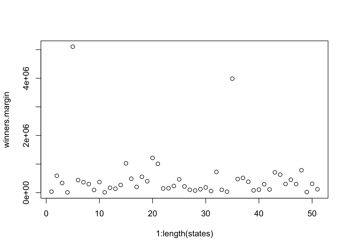
Again, why is this wrong?
states <- unique(pres$state)
biden.votes <- rep(NA, length(states))
trump.votes <- rep(NA, length(states))
winners.margin <- rep(NA, length(states))
for(i in 1:length(states)){
  biden.votes[i] <- sum(pres$biden.votes[pres$state==states[i]])
  trump.votes[i] <- sum(pres$trump.votes[pres$state==states[i]])

  if(biden.votes[i] >trump.votes[i]){
    winners.margin[i] <- biden.votes[i] - trump.votes[i]
  }

  winners.margin[i] <- trump.votes[i] - biden.votes[i]

}

plot(1:length(states), winners.margin)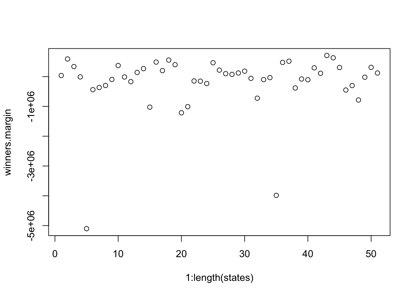
Because I’ve omitted the else, for this code we are calculating the biden margin in states that Biden won, but then immediately over-riding that with the trump margin. in other words: the Trump margin gets calcualted for every state, not just the ones Trump won.
10.1.1 Probability example
One of the most famous probability problems of all time is the “Monty Hall” problem, designed after an old game show. This show is, like, older than me.
You are on a game show and must choose one of three doors, where one conceals a new car and two conceal goats. After you randomly choose one door, the host of the game show, Monty, opens a different door, which does not conceal a car. Then, Monty asks you if you would like to switch to the unopened third door. You will win the new car if it is behind the door of your final choice. Should you switch, or stay with your original choice?
At the start of the game you pretty clealy have an unconditional probability of selecting the car of \(1/3\). There are three outcomes, and only one of them is the car. And it’s tempting to think that your odds don’t change once a goat is revealed. That is, it feels like the outcome of staying and switching are each 50%, so it doesn’t really matter what you do. Most people, when playing this game, choose to stay with their original choice.
The key to understanding the “trick” to this game, is that Monty knows where the car is, and never reveals the car in the second stage of the game. If your initial selection is one of the goats, Monty has to reveal the second goat, and not the car. In that case (where you initially select a goat), switching always wins you the car.
Let’s write this out in R. Like other probability problems, i’m going to start by writing this out once, before putting it in a loop so we can calculate the long term probabilities. We want to know, for a given initial random selection, what happens if we stay and what happens if we switch.
set.seed(19104)
stay <- NA
switch <- NA
#Stage one of game, randomly select a door
selection <- sample(c("goat","goat","car"),1)
selection
#> [1] "goat"
#We selected a goat, Monty knows this, but we don't.
#If we stay we get what we selected
stay <- selection
#The outcome of switching depends on our selection.
#If we selected a goat initially, monty reveals the other goat
#and swithing gets us a car.
#If we selected a car initially, monty reveals one of the two goats
#and swithing gets us a goat
if(selection=="goat"){
switch <- "car"
} else if (selection=="car"){
switch <- "goat"
}
stay
#> [1] "goat"
switch
#> [1] "car"
In this first simulation where we initially select a goat, staying gets us a goat, and switching gets us a car.
What are the relative success rates of these two strategies (stay and switch) long term? Let’s put this code in a loop to determine that:
stay <- NA
switch <- NA

for(i in 1:10000){
  #Stage one of game, randomly select a door
  selection <- sample(c("goat","goat","car"),1)
  selection
  #We selected a goat, Monty knows this, but we don't.
  #If we stay we get what we selected
  stay[i] <- selection
  #The outcome of switching depends on our selection.
  #If we selected a goat initially, monty reveals the other goat
  #and swithing gets us a car.
  #If we selected a car initially, monty reveals one of the two goats
  #and swithing gets us a goat
  if(selection=="goat"){
    switch[i] <- "car"
  } else if (selection=="car"){
    switch[i] <- "goat"
  }
}
mean(stay=="car")
#> [1] 0.3366
mean(switch=="car")
#> [1] 0.6634
Staying with your initial choice every time gets you the car 1/3 of the time, switching every time gets you the car 2/3 of the time.
10.2 Functions
Functions take a specific set of inputs and produce a specific set out of outputs.
That might sound confusing, you have already been using functions constantly. Every time you write mean(), sum(), length(), table(), or head() you are calling a function. Someone, at some point, wrote the code that makes mean() work, and packaged it up so that all you have to do is give it a vector (an input) and it gives you back the mean (the output).
In this section we are going to learn how to write our own functions. This is one of the most powerful things you can do in R, and it is going to be especially important when we move into the tidyverse in the next two chapters.
10.2.1 Why Write Functions?
Here’s the basic idea: if you find yourself copy-pasting the same chunk of code and just changing one or two things each time, you should probably write a function instead.
Let’s pretend that there is no function called mean. To calculate a mean we add up all the numbers in a vector and divide by the total number of entries.
So if we had the following vector, we can mathematically get the mean by doing:
But that would be very inefficient. Instead, what we can do with a function is say: I am going to give you a vector, take that vector and sum up all the values and divide by the length, then return the output.
10.2.2 The Basics
A function in R has three parts: a name, arguments (the inputs), and a body (the code that runs). Here is the simplest possible function:
say.hello <- function(){
  print("Hello!")
}
Let’s break this down. say.hello is the name – this is what we will type to call the function, just like we type mean to call the mean function. The function() part tells R “I am defining a function.” The curly braces {} contain the body – the code that runs when you call the function. In this case, all it does is print “Hello!”.
To call the function:
say.hello()
#> [1] "Hello!"
Note the parentheses. If you forget them, R doesn’t run the function – it just tells you that the function exists:
say.hello
#> function ()
#> {
#>     print("Hello!")
#> }
That’s not what we want. Always include the parentheses when you want to actually run a function.
10.2.3 Adding Arguments
A function that does the same thing every time isn’t very useful. The real power comes from giving functions arguments – inputs that change what the function does.
To continue our example, let’s write our own function for calculating the mean:
The input into this function is vec, which will be a vector of numbers. The function sums that vector and divides by it’s length, giving us the mean.
Now we can set vecequal to any vector of numbers and it will calculate the mean:
x <- 1:175
new.mean(vec=x)
#> [1] 88
R will automatically treat what you put in parentheses as the first argument, so we can shortcut this to:
new.mean(x)
#> [1] 88
#To show it works with other things
y <- 4:17
new.mean(y)
#> [1] 10.5
We can put as many arguments as we want into a function. For example, we may want a function that calculates vote share given a candidate share and total votes.
pres$total.votes <- pres$biden.votes + pres$trump.votes + pres$other.votes

#To create a vote share, in percent:

vs <- round(100*(pres$biden.votes/pres$total.votes),2)
head(vs)
#> [1] 47.54 24.34 29.45 26.31 34.57 37.24

#Put that into a function

vote.share <- function(cand.votes, total.votes){
round(100*(cand.votes/total.votes),2)
}


vs <- vote.share(cand.votes=pres$biden.votes, total.votes = pres$total.votes)
head(vs)
#> [1] 47.54 24.34 29.45 26.31 34.57 37.24

#R will assume first you put is first argument, second thing is second argument etc.
vs <- vote.share(pres$trump.votes, pres$total.votes)
head(vs)
#> [1] 48.00 72.12 66.77 70.23 60.31 58.67
We are not limited to putting just vectors into functions.
Let’s say we have a reduced datat-set that is just the vote columns.
votes <- pres[,4:7]
head(votes)
#>   biden.votes trump.votes other.votes total.votes
#> 1        3477        3511         326        7314
#> 2        2727        8081         397       11205
#> 3        3130        7096         402       10628
#> 4        2957        7893         388       11238
#> 5        2666        4652         395        7713
#> 6        4261        6714         468       11443
We can write a function that will “standardize” these variables, that is, divide each entry by the standard deviation of the variable.
As always, it’s best to write this first outside the function, and then to put it in function form.
#Preserve original data by creating a new dataset
tmp <- votes
#Loop across the columns. For each column divide by that column's standard deviation
for(i in 1:ncol(tmp)){
  tmp[,i] <- tmp[,i]/sd(tmp[,i])
}
head(tmp)
#>   biden.votes trump.votes other.votes total.votes
#> 1  0.04316422  0.07710407   0.1395737  0.05873340
#> 2  0.03385356  0.17746455   0.1699717  0.08997919
#> 3  0.03885649  0.15583324   0.1721124  0.08534572
#> 4  0.03670883  0.17333593   0.1661184  0.09024419
#> 5  0.03309629  0.10216125   0.1691154  0.06193748
#> 6  0.05289696  0.14744425   0.2003697  0.09189039
#Standardized variables have a sd of 1 by definition:
sd(tmp$biden.votes)
#> [1] 1

#Put this in a function
stdrdz <- function(dat){
  for(i in 1:ncol(dat)){
    dat[,i] <- dat[,i]/sd(dat[,i])
  }
}

tmp <- stdrdz(votes)
head(tmp)
#> NULL
#Nothing here??
Ok, we followed our previous steps but nothing showed up when we ran the function…. What’s the problem here.
When we are writing a function that works on a full dataset, we need to explicitly tell R that we want the function to spit back out the dataset dat at the end of the function. We can do that by using return()
stdrdz <- function(dat){
  for(i in 1:ncol(dat)){
    dat[,i] <- dat[,i]/sd(dat[,i])
  }
  #Explicitly say: return dat as the output of this function
  return(dat)
}

tmp <- stdrdz(votes)
head(tmp)
#>   biden.votes trump.votes other.votes total.votes
#> 1  0.04316422  0.07710407   0.1395737  0.05873340
#> 2  0.03385356  0.17746455   0.1699717  0.08997919
#> 3  0.03885649  0.15583324   0.1721124  0.08534572
#> 4  0.03670883  0.17333593   0.1661184  0.09024419
#> 5  0.03309629  0.10216125   0.1691154  0.06193748
#> 6  0.05289696  0.14744425   0.2003697  0.09189039
Sometimes when we standardize variables we also want to “mean-center” them. In that operation we subtract the mean of the variable from each value before dividing by the standard deviation. This results in a variable that has mean 0 and standard deviation 1. (This will become really helpful when we get to regression, for reasons that will only be obvious then. )
How can we edit our function to sometimes mean center the variable, when that’s what we want?
The word sometimes should cue you to an if statement.
We can add an argument to our function that is true if we want mean centered variables and false if we do not:
stdrdz <- function(dat, mean.centered){
  if(mean.centered==T){
    for(i in 1:ncol(dat)){
      dat[,i] <- (dat[,i]-mean(dat[,i]))/sd(dat[,i])
    }
  }else {
    for(i in 1:ncol(dat)){
      dat[,i] <- dat[,i]/sd(dat[,i])
    }
  }
  #Explicitly say: return dat as the output of this function
  return(dat)
}

tmp <- stdrdz(votes, mean.centered = T)
head(tmp)
#>   biden.votes trump.votes other.votes total.votes
#> 1  -0.1845510  -0.2829348  -0.1354869  -0.2253795
#> 2  -0.1938617  -0.1825743  -0.1050890  -0.1941337
#> 3  -0.1888587  -0.2042056  -0.1029483  -0.1987672
#> 4  -0.1910064  -0.1867029  -0.1089422  -0.1938687
#> 5  -0.1946189  -0.2578776  -0.1059452  -0.2221754
#> 6  -0.1748183  -0.2125946  -0.0746910  -0.1922225
mean(tmp$biden.votes)
#> [1] 1.210306e-17

tmp <- stdrdz(votes, mean.centered = F)
head(tmp)
#>   biden.votes trump.votes other.votes total.votes
#> 1  0.04316422  0.07710407   0.1395737  0.05873340
#> 2  0.03385356  0.17746455   0.1699717  0.08997919
#> 3  0.03885649  0.15583324   0.1721124  0.08534572
#> 4  0.03670883  0.17333593   0.1661184  0.09024419
#> 5  0.03309629  0.10216125   0.1691154  0.06193748
#> 6  0.05289696  0.14744425   0.2003697  0.09189039
mean(tmp$biden.votes)
#> [1] 0.2277152
Now, that’s a lot of squiggly brackets! When I wrote that, just now, I had to carefully go through to make sure all the squiggly brackets were in the right place. Two tips on this: (1) if you highlight a piece of code and then press cmd+I on mac or ctrl+I on windows, it will indent all of the code in a way that is easier to read; (2) This is hard because it’s hard. This is something I will have to say to you occasionally in this course and future courses. Some things are just hard and take some repetition to get right.
One final piece of customization to this function is that we can set defaults for arguments. We can technically do this for any of the arguments, although we will most commonly use them for arguments that are T or F. If we re-define our standardize function we can explicitly set mean.centered=T in the definition, and that will become the default:
stdrdz <- function(dat, mean.centered=T){
  if(mean.centered==T){
    for(i in 1:ncol(dat)){
      dat[,i] <- (dat[,i]-mean(dat[,i]))/sd(dat[,i])
    }
  }else {
    for(i in 1:ncol(dat)){
      dat[,i] <- dat[,i]/sd(dat[,i])
    }
  }
  #Explicitly say: return dat as the output of this function
  return(dat)
}

#By default mean centers:
tmp <- stdrdz(votes)
mean(tmp$biden.votes)
#> [1] 1.210306e-17

#Can override:
tmp <- stdrdz(votes, mean.centered=F)
mean(tmp$biden.votes)
#> [1] 0.2277152
10.3 Use case
Functions are incredibly helpful whenever you are repeating the same thing many times.
Let’s say we are working with the pres data and we want to be able to generate state summary tables for any state.
I want to be able to put in "AL", and have it output a nice table of the results in Alabama. That table will have the name of the state, the winner of the state, the Democratic and Republican percent of the vote, and the total votes.
The way we want to do this is to first set this up for one state, and then generalize that into a function:
#The things we want to generate are state, winner, dem perc, rep perc, and total votes
input.state <- "AL"

#Define state for output
state <- input.state

#Calculate the statewide dem and rep perc
dem.perc <- round(100*(sum(pres$biden.votes[pres$state==input.state])/sum(pres$total.votes[pres$state==input.state])),1)
rep.perc <- round(100*(sum(pres$trump.votes[pres$state==input.state])/sum(pres$total.votes[pres$state==input.state])),1)

#Use and if/else statement to define the winner based on the relative size of dem and rep percent, which we just defined
#No states are ties
if(dem.perc>rep.perc){
  winner = "Biden"
} else {
  winner = "Trump"
  }

#Define total votes
total.votes <- sum(pres$total.votes[pres$state==input.state])

#Make output dataframe
out <- cbind.data.frame(state, winner, dem.perc, rep.perc, total.votes)

names(out) <- c("State", "Winner", "Democratic Percent", "Republican Percent", "Total Votes")

#Need kableExtra package for this part to work:
kableExtra::kable(out)| State | Winner | Democratic Percent | Republican Percent | Total Votes |
|---|---|---|---|---|
| AL | Trump | 36.6 | 62 | 2323282 |
I have written that code so that I can, if I want, just copy and paste it and change input.state to a different state and get the right output. So if I copy and paste and change it to PA:
#The things we want to generate are state, winner, dem perc, rep perc, and total votes
input.state <- "PA"

#Define state for output
state <- input.state

#Calculate the statewide dem and rep perc
dem.perc <- round(100*(sum(pres$biden.votes[pres$state==input.state])/sum(pres$total.votes[pres$state==input.state])),1)
rep.perc <- round(100*(sum(pres$trump.votes[pres$state==input.state])/sum(pres$total.votes[pres$state==input.state])),1)

#Use and if/else statement to define the winner based on the relative size of dem and rep percent, which we just defined
#No states are ties
if(dem.perc>rep.perc){
  winner = "Biden"
} else {
  winner = "Trump"
  }

#Define total votes
total.votes <- sum(pres$total.votes[pres$state==input.state])

#Make output dataframe
out <- cbind.data.frame(state, winner, dem.perc, rep.perc, total.votes)

names(out) <- c("State", "Winner", "Democratic Percent", "Republican Percent", "Total Votes")

#Need kableExtra package for this part to work:
kableExtra::kable(out)| State | Winner | Democratic Percent | Republican Percent | Total Votes |
|---|---|---|---|---|
| PA | Biden | 50 | 48.8 | 6915220 |
It will produce the right output. But if I am writing a report and want to keep outputting these small tables, it would be extremely inefficient to run this big block of code everytime! Instead, let’s put this inside a function where the argument is the input state:
state.table <- function(input.state){
  #Define state for output
  state <- input.state

  #Calculate the statewide dem and rep perc
  dem.perc <- round(100*(sum(pres$biden.votes[pres$state==input.state])/sum(pres$total.votes[pres$state==input.state])),1)
  rep.perc <- round(100*(sum(pres$trump.votes[pres$state==input.state])/sum(pres$total.votes[pres$state==input.state])),1)

  #Use and if/else statement to define the winner based on the relative size of dem and rep percent, which we just defined
  #No states are ties
  if(dem.perc>rep.perc){
    winner = "Biden"
  } else {
    winner = "Trump"
  }

  #Define total votes
  total.votes <- sum(pres$total.votes[pres$state==input.state])

  #Make output dataframe
  out <- cbind.data.frame(state, winner, dem.perc, rep.perc, total.votes)

  names(out) <- c("State", "Winner", "Democratic Percent", "Republican Percent", "Total Votes")
  #Output is that table
  return(out)
}
Now that function is created, if I want to print the state results for Texas all I have to do is:
kableExtra::kable(state.table("TX"))| State | Winner | Democratic Percent | Republican Percent | Total Votes |
|---|---|---|---|---|
| TX | Trump | 46.5 | 52.1 | 11315056 |
kableExtra::kable(state.table("WI"))| State | Winner | Democratic Percent | Republican Percent | Total Votes |
|---|---|---|---|---|
| WI | Biden | 49.5 | 48.8 | 3297352 |
That is way cleaner code because I only have the big chunk of messy code once, and then I just have to call the function anytime I want a table.
There is one more, completely optional, step. We can actually save the function in a different R script and then load that function in by calling that R script using source(). What source() does is runs, in the background, an external R script. This is helpful because it keeps the messy R code out of our file completely.
I have saved the state.table() function in an R script which I have uploaded to the github. You can download that R script, but it is literally just what is above saved to a seperate file. We can use source and the link to read that file and that function will now be available to us. Usually we would do this with an R file saved on our computer, but to make it so you can all do this, i’ve uploadrd it to github.
#First remove the function so we can show source() works
rm(state.table)

#Read the file from github.
source("https://github.com/marctrussler/IDS-Data/raw/refs/heads/main/StateTable.R")

#Use the function
kableExtra::kable(state.table("MN"))| State | Winner | Democratic Percent | Republican Percent | Total Votes |
|---|---|---|---|---|
| MN | Biden | 52.4 | 45.3 | 3277171 |
10.3.1 Looking Ahead
In the next two chapters we are going to learn the tidyverse, which is built entirely around this idea of packaging operations into functions. Now that you know how to write your own functions in base R, you’ll be able to plug them right into that workflow. The tidyverse doesn’t do anything magical – it’s just functions all the way down, and now you know how to make your own.