16 Final Review
The final exam will be cumulative because the material we have learned is cumulative. You can’t be good at the stuff in the second half of the class without understanding what happened in the first half.
Accordingly: the best way to review for the final exam will be to read the notes in this textbook (though at this point you should be able to mostly focus on the second half, assuming you already have the first half down) and to carefully go through the problem set questions. Just like the midterm, it’s helpful to literally write out the code that is in the textbook. The reps will help you avoid the kind of small errors that can derail you in a timed exam.
The post-midterm material is different than the pre-midterm material in two ways. First, it covers more chapters. Second, the regression material at the end is more conceptually demanding than anything we covered before the midterm. The questions there are less about getting code to work and more about correctly interpreting what the regression is telling you. Practice writing out interpretations in plain English.
Problem sets 3 and 4 cover the bulk of the material, and the regression question covers regression specifically. As before: the final exam questions will be straight-forward applications of in-class examples and problem set questions. There will be nothing surprising.
My tips from the midterm review apply here too: knit your rmarkdown often, read every question fully, pay attention to the words I use in questions, and put something down for absolutely every question.
16.1 Broad view of the course (post-midterm)
Brief notes on each chapter to give a sense of what I want you to take away. The following is definitely not sufficient for studying.
16.1.1 Collecting and Merging Data
Merging requires absolute clarity in terms of unit of analysis: are you working with individuals, counties, countries, country-years, candidate-districts, candidate-district-years?
- Merging two datasets together with
merge(), using a shared identifier.
acs <- rio::import("https://github.com/marctrussler/IDS-Data/raw/main/ACSCountyData.csv", trust=T)

#A small dataset to merge in
income.rank <- data.frame(
  county.fips = acs$county.fips,
  income.rank = rank(-acs$median.income)
)

merged <- merge(acs, income.rank, by="county.fips")
head(merged[,c("county.name","median.income","income.rank")])
#>      county.name median.income income.rank
#> 1 Autauga County         58786       708.0
#> 2 Baldwin County         55962       921.0
#> 3 Barbour County         34186      2964.5
#> 4    Bibb County         45340      2071.5
#> 5  Blount County         48695      1715.0
#> 6 Bullock County 32152 3027.0- The
all.xandall.yarguments control which non-matching rows you keep.
#Keep all rows from x even if no match in y
merge(x, y, by="id", all.x=TRUE)
One-to-one and one-to-many merges work cleanly. Many-to-many merges don’t work and indicate that you need a second merge variable.
FIPS codes (and other identifiers with leading zeros) get destroyed when read in as numbers. You may have to use
as.character()to pad them back out, or import as character to begin with. More broadly: you need to do work before a merge to determine which cases do not merge, and why.The ecological inference fallacy: a relationship that exists at the aggregate level does not necessarily hold at the individual level. If counties with more transit use have higher COVID rates, that does not mean transit users themselves had higher COVID rates.
16.1.2 If Statements and Functions
if lets your code take different paths based on a condition. function() lets you bundle code you do repeatedly into a single named tool.
- Basic conditional flow.
x <- 10

if(x > 5){
  print("Big")
} else if(x > 0){
  print("Small but positive")
} else {
  print("Negative or zero")
}
#> [1] "Big"- Writing your own function with arguments and a
return().
standardize <- function(x){
  z <- (x - mean(x, na.rm=T))/sd(x, na.rm=T)
  return(z)
}

#Test it
standardize(c(1,2,3,4,5))
#> [1] -1.2649111 -0.6324555 0.0000000 0.6324555 1.2649111- Functions can have default values for their arguments.
trim.mean <- function(x, trim=0.1){
  return(mean(x, trim=trim, na.rm=T))
}

trim.mean(acs$median.income)
#> [1] 50248.51
trim.mean(acs$median.income, trim=0.25)
#> [1] 49872.21- Using a function inside a
for()loop to simulate probability. The Monty Hall problem is the classic example: simulate the game many times under both strategies, see which wins more often.
#Simulate one round where you switch
monty.switch <- function(){
  doors <- c("car","goat","goat")
  doors <- sample(doors)
  pick <- 1
  reveal <- which(doors=="goat" & 1:3 != pick)[1]
  switch.to <- which(1:3 != pick & 1:3 != reveal)
  return(doors[switch.to]=="car")
}

results <- rep(NA, 10000)
for(i in 1:10000){
  results[i] <- monty.switch()
}
mean(results)
#> [1] 0.6653
16.1.3 Tidyverse I
The tidyverse provides a set of “verbs” that operate on data frames. Each verb returns a data frame, which means you can chain them together with the pipe |>.
- The six core verbs.
library(tidyverse)

#filter() keeps rows
acs |>
  filter(state.full=="Pennsylvania") |>
  head()
#>     V1 county.fips     county.name   state.full state.abbr
#> 1 2245       42015 Bradford County Pennsylvania         PA
#> 2 2246       42017    Bucks County Pennsylvania         PA
#> 3 2247       42013    Blair County Pennsylvania         PA
#> 4 2248       42083   McKean County Pennsylvania         PA
#> 5 2249       42085   Mercer County Pennsylvania         PA
#> 6 2250       42087  Mifflin County Pennsylvania         PA
#>   state.alpha state.icpsr census.region population
#> 1          38          14     northeast      61304
#> 2          38          14     northeast     626370
#> 3          38          14     northeast     123842
#> 4          38          14     northeast      41806
#> 5          38          14     northeast     112630
#> 6          38          14     northeast      46362
#>   population.density percent.senior percent.white
#> 1           53.42781       20.26295      96.92353
#> 2         1036.30200       17.61275      88.01555
#> 3          235.53000       19.79781      95.50799
#> 4           42.69485       18.51409      94.48405
#> 5          167.45910       20.70674      91.22969
#> 6          112.79050       20.77779      96.88322
#>   percent.black percent.asian percent.amerindian
#> 1     0.4404280     0.6769542         0.06361738
#> 2     4.0017881     4.6973833         0.16475885
#> 3     1.6214208     0.6992781         0.03391418
#> 4     2.4876812     0.4449122         0.06697603
#> 5     5.6698926     0.6889816         0.10920714
#> 6     0.7915966     0.1898106         0.15745654
#>   percent.less.hs percent.college unemployment.rate
#> 1       11.085675        17.84021          4.808069
#> 2        6.144487        40.46496          4.524462
#> 3        9.070472        20.80933          4.961147
#> 4        8.908716        18.14864          6.829542
#> 5       10.161785        22.55270          5.271703
#> 6       14.792334        12.47843          3.598866
#>   median.income   gini median.rent percent.child.poverty
#> 1         51457 0.4310         711             17.012323
#> 2         86055 0.4480        1207              7.358998
#> 3         47969 0.4448         711             19.575034
#> 4         46953 0.4475         644             27.077236
#> 5         48768 0.4381         679             24.827619
#> 6         47526 0.4144         665             23.594624
#>   percent.adult.poverty percent.car.commute
#> 1             11.132679            90.12223
#> 2              5.743422            88.75924
#> 3             14.600937            91.58161
#> 4             16.563244            91.10273
#> 5             13.507259            90.04547
#> 6             13.347636            90.67850
#>   percent.transit.commute percent.bicycle.commute
#> 1               0.2475153              0.27036290
#> 2               3.4039931              0.16052502
#> 3               1.1913318              0.18328182
#> 4               0.9152430              0.17750166
#> 5               0.4175279              0.08887970
#> 6               0.3038048              0.05786758
#>   percent.walk.commute average.commute.time
#> 1             3.625148                   23
#> 2             1.717094                   30
#> 3             3.056494                   20
#> 4             3.372532                   22
#> 5             3.577925                   21
#> 6             2.956069                   24
#>   percent.no.insurance
#> 1             6.692875
#> 2             4.212366
#> 3             5.240548
#> 4             4.568722
#> 5             6.158217
#> 6            12.339847

#select() keeps columns
acs |>
  select(county.name, state.full, median.income) |>
  head()
#>       county.name state.full median.income
#> 1   Etowah County    Alabama         44023
#> 2  Winston County    Alabama         38504
#> 3 Escambia County    Alabama         35000
#> 4  Autauga County    Alabama         58786
#> 5  Baldwin County    Alabama         55962
#> 6  Barbour County    Alabama         34186

#mutate() creates or modifies columns
acs |>
  mutate(income.k = median.income/1000) |>
  select(county.name, income.k) |>
  head()
#>       county.name income.k
#> 1   Etowah County   44.023
#> 2  Winston County   38.504
#> 3 Escambia County   35.000
#> 4  Autauga County   58.786
#> 5  Baldwin County   55.962
#> 6  Barbour County   34.186

#arrange() sorts
acs |>
  arrange(desc(median.income)) |>
  select(county.name, median.income) |>
  head()
#>          county.name median.income
#> 1     Loudoun County        136268
#> 2  Falls Church city        124796
#> 3     Fairfax County        121133
#> 4      Howard County        117730
#> 5   Arlington County        117374
#> 6 Santa Clara County        116178

#group_by() + summarize() collapses data
acs |>
  group_by(census.region) |>
  summarize(mean.income = mean(median.income, na.rm=T))
#> # A tibble: 4 × 2
#>   census.region mean.income
#>   <chr>               <dbl>
#> 1 midwest            53487.
#> 2 northeast          61994.
#> 3 south              47323.
#> 4 west               55591.

#distinct() returns unique values
acs |>
  distinct(state.full) |>
  head()
#>   state.full
#> 1    Alabama
#> 2     Alaska
#> 3    Arizona
#> 4   Arkansas
#> 5 California
#> 6   Colorado
The pipe
|>takes the thing on its left and feeds it as the first argument of the function on its right. This meansmean(x)is the same asx |> mean().select()has helpers:starts_with(),ends_with(),contains(). Useful when you have many similarly-named variables.
acs |>
  select(starts_with("percent")) |>
  head()
#>   percent.senior percent.white percent.black percent.asian
#> 1       18.33804      80.34856    15.7491330     0.7179009
#> 2       21.05550      96.33927     0.3769634     0.1298429
#> 3       17.34891      61.87045    31.9331333     0.3616588
#> 4       14.58333      76.87862    19.1394928     1.0289855
#> 5       19.54043      86.26620     9.4970376     0.8072770
#> 6       17.97378      47.38189    47.5758281     0.3723528
#>   percent.amerindian percent.less.hs percent.college
#> 1          0.7295583       15.483020        17.73318
#> 2          0.3895288       21.851723        13.53585
#> 3          3.8496571       18.455613        12.65935
#> 4          0.2880435       11.311414        27.68929
#> 5          0.7313545        9.735422        31.34588
#> 6          0.2792646       26.968580        12.21592
#>   percent.child.poverty percent.adult.poverty
#> 1              30.00183              15.42045
#> 2              23.91744              15.83042
#> 3              33.89582              23.50816
#> 4              22.71976              14.03953
#> 5              13.38019              10.37312
#> 6              47.59704              25.40757
#>   percent.car.commute percent.transit.commute
#> 1            94.28592              0.20813669
#> 2            94.63996              0.38203288
#> 3            98.54988              0.00000000
#> 4            95.15310              0.10643524
#> 5            91.71079              0.08969591
#> 6            94.22581              0.25767159
#>   percent.bicycle.commute percent.walk.commute
#> 1              0.08470679            0.8373872
#> 2              0.00000000            0.3473026
#> 3              0.06667222            0.4250354
#> 4              0.05731128            0.6263304
#> 5              0.05797419            0.6956902
#> 6              0.00000000            2.1316468
#>   percent.no.insurance
#> 1            10.357590
#> 2            12.150785
#> 3            14.308294
#> 4             7.019928
#> 5            10.025612
#> 6 9.921651-
group_by()followed bysummarize()is the workhorse pattern. You group the data, you compute summaries within each group, you get one row per group out.
16.1.4 Tidyverse II
The second tidyverse chapter adds joins (the tidyverse version of merge()), conditional column creation, and across() for applying a function to many columns at once.
- Joins.
left_join()keeps all rows from the left dataset;inner_join()keeps only rows that match in both.
left_join(acs, income.rank, by="county.fips")
inner_join(acs, income.rank, by="county.fips")-
if_else()for two-way conditional assignment,case_when()for many-way.
acs |>
  mutate(income.cat = case_when(
    median.income < 40000 ~ "Low",
    median.income < 70000 ~ "Middle",
    .default = "High"
  )) |>
  count(income.cat)
#>   income.cat    n
#> 1       High  272
#> 2        Low  542
#> 3 Middle 2328across()applies a function to multiple columns. Useful for standardizing or recoding many variables at once.The
\(x)syntax lets you write a small inline function insideacross().
acs |>
  mutate(across(c(median.income, percent.white, percent.senior), \(x) (x-mean(x, na.rm=T))/sd(x,na.rm=T))) |>
  select(median.income, percent.white, percent.senior) |>
  head()
#>   median.income percent.white percent.senior
#> 1    -0.5516966    -0.1604264   -0.005655642
#> 2    -0.9544403     0.7874248    0.586911476
#> 3    -1.2101414    -1.2557185   -0.221346836
#> 4     0.5256193    -0.3661070   -0.824407239
#> 5     0.3195405     0.1903426    0.256535927
#> 6    -1.2695423    -2.1145290   -0.085087126
16.1.5 Writing and Visualizing: ggplot2 Grammar
I’m not going to test you on the writing material directly, but the principles (know what you want to say, get to the point, keep it simple) apply to every short answer you write on the exam.
Likewise: nothing on the exam will require you to use ggplot instead of a base R plot. However, here is a basic review of how it works.
For ggplot, the thing to internalize is the grammar. Every plot has three required pieces:
- Data: a data frame.
-
Aesthetics (
aes()): a mapping from variables in the data to visual properties (x, y, color, fill, size). -
Geoms: the actual shapes drawn (
geom_point,geom_col,geom_histogram, etc.).
elect <- rio::import("https://github.com/marctrussler/IDS-Data/raw/main/VizData.Rds")- The basic syntax.
ggplot()takes data and aesthetics. Geoms get added with+.
ggplot(elect, aes(x = p.white, y = plean.20)) +
  geom_point()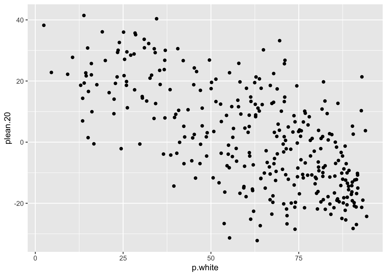
- Layering. The order you add geoms is the order they are drawn.
ggplot(elect, aes(x = p.white, y = plean.20)) +
  geom_point(alpha = 0.3) +
  geom_smooth(method = "lm", color = "firebrick")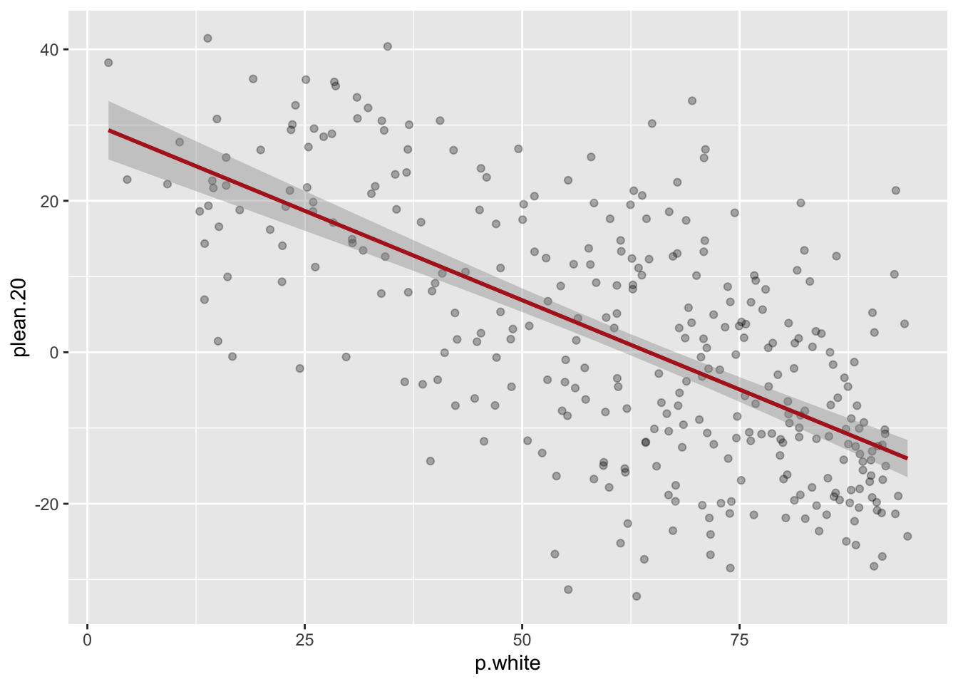
- The pipe-to-plot pattern: pipe a dataset (often after
filter()orgroup_by()/summarize()) directly intoggplot(). Once insideggplot()you switch from|>to+.
elect |>
  filter(!is.na(plean.20)) |>
  group_by(region) |>
  summarize(mean.lean = mean(plean.20)) |>
  ggplot(aes(x = region, y = mean.lean)) +
  geom_col(fill = "steelblue")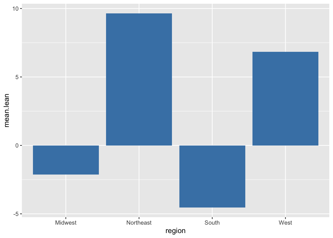
#Color varies by a variable
geom_point(aes(color = region))

#Color is fixed for all points
geom_point(color = "steelblue")
Common geoms:
geom_point()(scatterplot),geom_smooth()(smoothed line),geom_col()(bar chart from summarized data),geom_histogram()(one continuous variable),geom_density()(smoothed histogram),geom_boxplot()(distribution by group),geom_hline()/geom_vline()(reference lines).facet_wrap(~variable)splits a plot into small multiples by a categorical variable.
16.1.6 Regression I
Regression is a method for summarizing the relationship between two (or more) variables with a line. The line is fit by Ordinary Least Squares: out of all possible lines, OLS picks the one that minimizes the sum of squared vertical distances between the line and the data points.
The basic equation for a regression line is:
\[\hat{y} = \alpha + \beta x_i \]
- \(\alpha\) is the intercept: the predicted value of \(y\) when \(x = 0\).
- \(\beta\) is the slope: the predicted change in \(y\) for a one-unit increase in \(x\).
Fitting and reading a regression in R.
m1 <- lm(median.income ~ percent.white, data=acs)
summary(m1)
#>
#> Call:
#> lm(formula = median.income ~ percent.white, data = acs)
#>
#> Residuals:
#>    Min     1Q Median     3Q    Max
#> -30877  -9028  -2133   5525  86564
#>
#> Coefficients:
#>               Estimate Std. Error t value Pr(>|t|)
#> (Intercept)   42350.29    1217.64  34.781  < 2e-16 ***
#> percent.white   111.15      14.37   7.737 1.36e-14 ***
#> ---
#> Signif. codes:
#> 0 '***' 0.001 '**' 0.01 '*' 0.05 '.' 0.1 ' ' 1
#>
#> Residual standard error: 13580 on 3139 degrees of freedom
#>   (1 observation deleted due to missingness)
#> Multiple R-squared:  0.01871,    Adjusted R-squared:  0.0184
#> F-statistic: 59.87 on 1 and 3139 DF,  p-value: 1.359e-14
16.1.6.1 Interpreting Coefficients
This is the part that matters. You need to be able to write out a sentence in plain English for any coefficient.
The intercept is the predicted \(y\) when all independent variables in the regression are zero. Often this is not a meaningful value (a county that has a median income of 0 does not exist; but, a county with a percent black of close to 0% probably exists).
The slope is the predicted change in \(y\) for a one-unit increase in \(x\). “One unit” means 1 integer, always. That means you have to pay attention to the scale your independent variable is on. If \(x\) is “percent White” then the unit is one percentage point. But if it was “proportion.white” then one unit would be from 0 to 100%. If \(x\) is “income in dollars” then the unit is one dollar. Pay attention to this — you may need to translate.
For the model above, the slope on percent.white is around $520, meaning: a one-percentage-point increase in the White share of a county is associated with about $520 higher median income.
16.1.6.2 Plotting the Line
plot(acs$percent.white, acs$median.income,
     xlab="Percent White", ylab="Median Income",
     pch=16, col=rgb(0,0,0,0.2))
abline(m1, col="firebrick", lwd=2)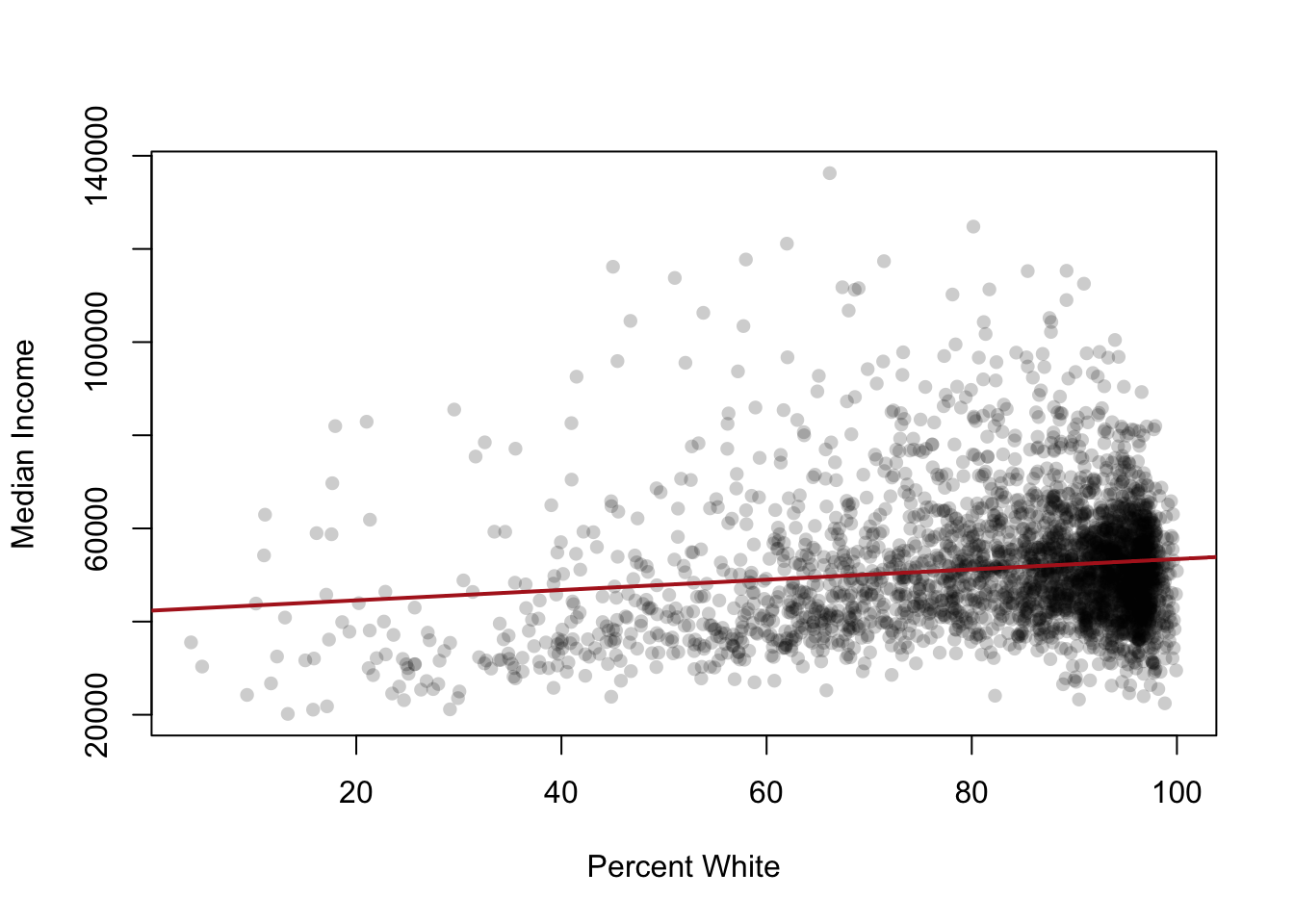
16.1.6.3 Hypothesis Tests on Coefficients
The summary() output shows a t-statistic and p-value for each coefficient. The null hypothesis is that the true coefficient is zero (no relationship). A small p-value (typically < 0.05) means we reject that null and conclude there is a relationship. Hypothesis tests are not a major feature of this course, so don’t worry too much about these.
16.1.6.4 Binary Predictors
When \(x\) is binary (0/1), the regression line connects two group means. The intercept is the mean of \(y\) in the group where \(x=0\). The slope is the difference between the two group means.
acs$urban <- ifelse(acs$population > 250000, 1, 0)
m2 <- lm(median.income ~ urban, data=acs)
coef(m2)
#> (Intercept)       urban
#>    50108.52    17283.14
The intercept here is the mean income for non-urban counties. The slope on urban is the difference in mean income between urban and non-urban counties.
16.1.6.5 Binary Outcomes (Linear Probability Model)
When \(y\) is binary, the regression coefficients are interpreted as changes in the probability that \(y=1\).
acs$rich <- ifelse(acs$median.income > 70000, 1, 0)
m3 <- lm(rich ~ percent.white, data=acs)
coef(m3)
#>   (Intercept) percent.white
#>  0.1665071185 -0.0009658663
The slope here is the change in the probability of being a “rich” county for a one-point increase in percent White. The Linear Probability Model can produce predicted probabilities outside [0,1], which is a known limitation, but it is fine for our purposes in this course.
16.1.7 Regression II
Multiple regression adds more predictors. The model becomes:
\[y_i = \alpha + \beta_1 x_{1i} + \beta_2 x_{2i} + \beta_3 x_{3i} + \ldots + \epsilon_i\]
Each coefficient is now interpreted as the effect of that variable holding the other variables in the model constant. This phrase is critical and will appear in every interpretation.
m4 <- lm(median.income ~ percent.white + percent.college, data=acs)
summary(m4)
#>
#> Call:
#> lm(formula = median.income ~ percent.white + percent.college,
#>     data = acs)
#>
#> Residuals:
#>    Min     1Q Median     3Q    Max
#> -37766  -5809   -834   5122  51406
#>
#> Coefficients:
#>                 Estimate Std. Error t value Pr(>|t|)
#> (Intercept)     20719.41     945.86   21.91   <2e-16 ***
#> percent.white     107.83      10.18   10.59   <2e-16 ***
#> percent.college  1015.42      18.20   55.80   <2e-16 ***
#> ---
#> Signif. codes:
#> 0 '***' 0.001 '**' 0.01 '*' 0.05 '.' 0.1 ' ' 1
#>
#> Residual standard error: 9620 on 3138 degrees of freedom
#>   (1 observation deleted due to missingness)
#> Multiple R-squared:  0.5075, Adjusted R-squared:  0.5072
#> F-statistic:  1617 on 2 and 3138 DF,  p-value: < 2.2e-16
The slope on percent.white here is the predicted change in median income for a one-point increase in percent White, holding percent with a college degree constant. Notice it is much smaller than the simple regression coefficient. That’s not an accident.
16.1.7.1 Omitted Variable Bias
When the simple regression coefficient changes after we control for another variable, it tells us something. The simple regression on percent.white was conflating the effect of being White with the effect of education (since these are correlated). The multiple regression separates them out.
A simple regression coefficient is biased whenever an omitted variable is:
- Correlated with the predictor in the model, AND
- A separate cause of the outcome.
The classic example: if you regress income on whether someone uses transit, you might find a negative relationship. But controlling for whether they live in a city makes that effect disappear or flip. The omitted variable (urbanicity) is correlated with transit use and separately affects income.
16.1.7.2 Post-Treatment Bias
The opposite mistake from omitted variable bias: do not control for variables that are caused by your predictor. If you want to know the effect of education on income, do not control for occupation — occupation is a consequence of education and controlling for it will partial out exactly the effect you are trying to measure.
16.1.7.3 Categorical Variables (Dummies)
When you include a categorical variable in lm(), R automatically converts it into a set of binary indicators (dummies), with one category dropped as the reference category.
m5 <- lm(median.income ~ as.factor(census.region), data=acs)
summary(m5)
#>
#> Call:
#> lm(formula = median.income ~ as.factor(census.region), data = acs)
#>
#> Residuals:
#>    Min     1Q Median     3Q    Max
#> -31506  -8314  -2055   5236  88945
#>
#> Coefficients:
#>                                   Estimate Std. Error
#> (Intercept)                        53486.5      399.9
#> as.factor(census.region)northeast   8507.4      968.2
#> as.factor(census.region)south      -6163.9      527.8
#> as.factor(census.region)west        2104.2      733.1
#>                                   t value Pr(>|t|)
#> (Intercept)                       133.743  < 2e-16 ***
#> as.factor(census.region)northeast   8.786  < 2e-16 ***
#> as.factor(census.region)south     -11.678  < 2e-16 ***
#> as.factor(census.region)west        2.870  0.00413 **
#> ---
#> Signif. codes:
#> 0 '***' 0.001 '**' 0.01 '*' 0.05 '.' 0.1 ' ' 1
#>
#> Residual standard error: 12990 on 3137 degrees of freedom
#>   (1 observation deleted due to missingness)
#> Multiple R-squared:  0.1023, Adjusted R-squared:  0.1015
#> F-statistic: 119.2 on 3 and 3137 DF, p-value: < 2.2e-16- The intercept is the mean of \(y\) in the reference category.
- Each other coefficient is the difference in mean \(y\) between that category and the reference category.
By default R picks the alphabetically first category as the reference. Use relevel() if you want to change it.
16.1.7.4 Substantive vs. Statistical Significance
A coefficient can be statistically significant (small p-value) but substantively trivial, or substantively large but not statistically significant. Always interpret both.
To compare effects across variables on different scales, multiply the coefficient by the standard deviation of the predictor. This gives the predicted change in \(y\) for a one-SD increase in \(x\), which is comparable across variables.