500*.45[1] 225Solve the following questions about the specified Binomial (\(B\)), Uniform (\(U\)) and Normal (\(N\)) random variables:
\(Y \sim B(n=500, \pi=.45)\)
500*.45[1] 225500*.45*(1-.45)[1] 123.75dbinom(150, 500, .45 )[1] 2.220032e-12pbinom(200, 500, .45)[1] 0.01356437pbinom(222, 500, .45) - pbinom(200, 500, .45) [1] 0.3980971We want to add up the probability of 201,202,203….222. We do not want to include the probability of 223 (so we start with all the probability up to including 222) and we do not want to include the probability of 200 (so we make sure to subtract off all the probability to the left of, and including, 200).
Visually:
out.nums <- c(195:200,223:227)
out.probs <- pbinom(out.nums, size=500, prob=.45)
in.nums <- 201:222
in.probs <- pbinom(in.nums, size=500, prob=.45)
plot(out.nums, out.probs, col="firebrick", pch=16, ylim=c(-.1, .7))
points(in.nums, in.probs, col="forestgreen", pch=16)
segments(190,-.05, 200, -.05)
segments(190,-.1, 222, -.1)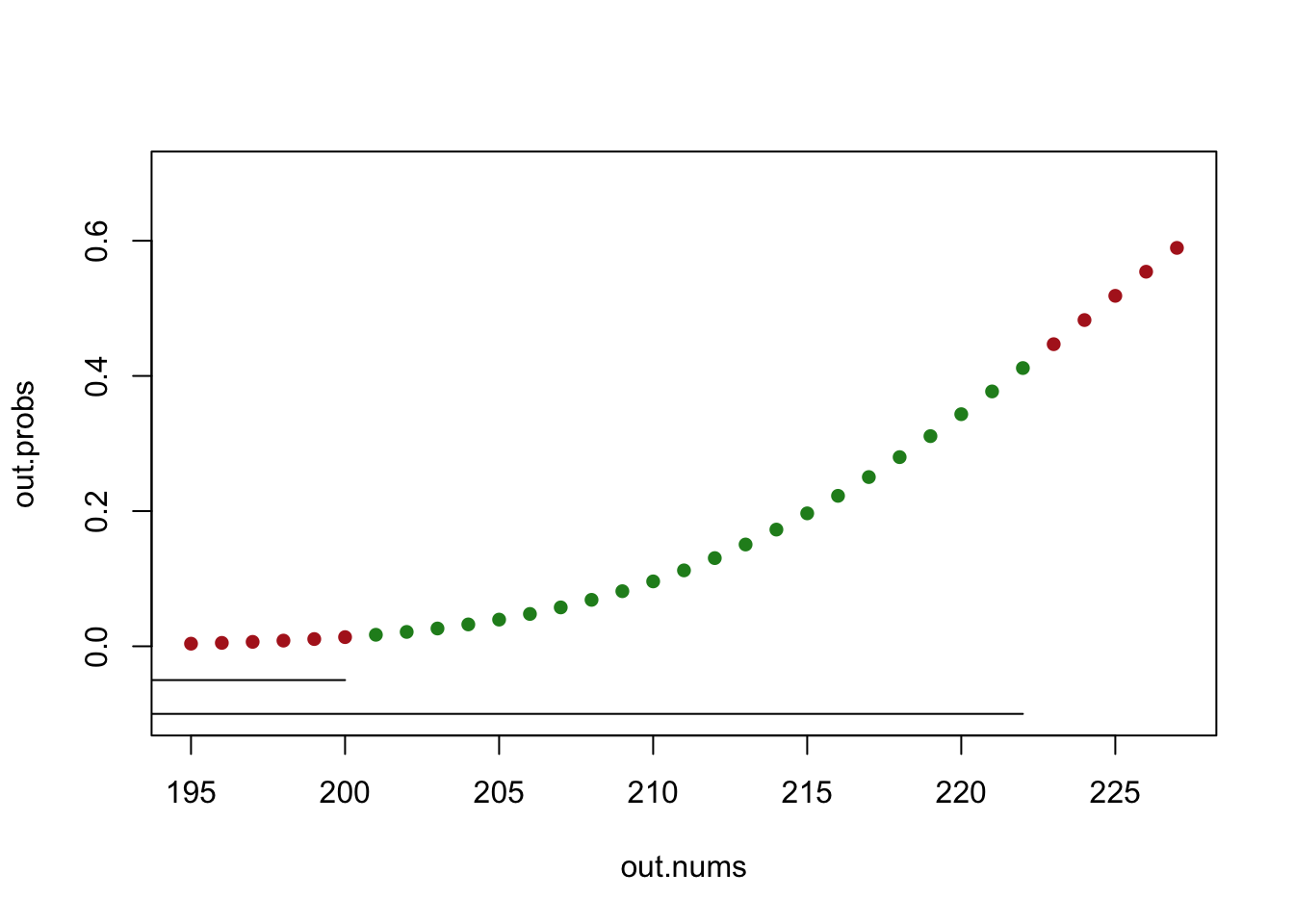
pbinom(223, 500, .45) - pbinom(199, 500, .45) [1] 0.436247We want to add up the probability of 200,201,202,203….223. We now want to include the exact probability of 223 (so we start with all the probability up to including 223) and we do want to include the probability of 200 (so we make sure not to subtract off its probability so we subtract off all the probability to the left of, and including, 199).
Visually:
out.nums <- c(195:199,224:227)
out.probs <- pbinom(out.nums, size=500, prob=.45)
in.nums <- 200:223
in.probs <- pbinom(in.nums, size=500, prob=.45)
plot(out.nums, out.probs, col="firebrick", pch=16, ylim=c(-.1, .7))
points(in.nums, in.probs, col="forestgreen", pch=16)
segments(190,-.05, 199, -.05)
segments(190,-.1, 223, -.1)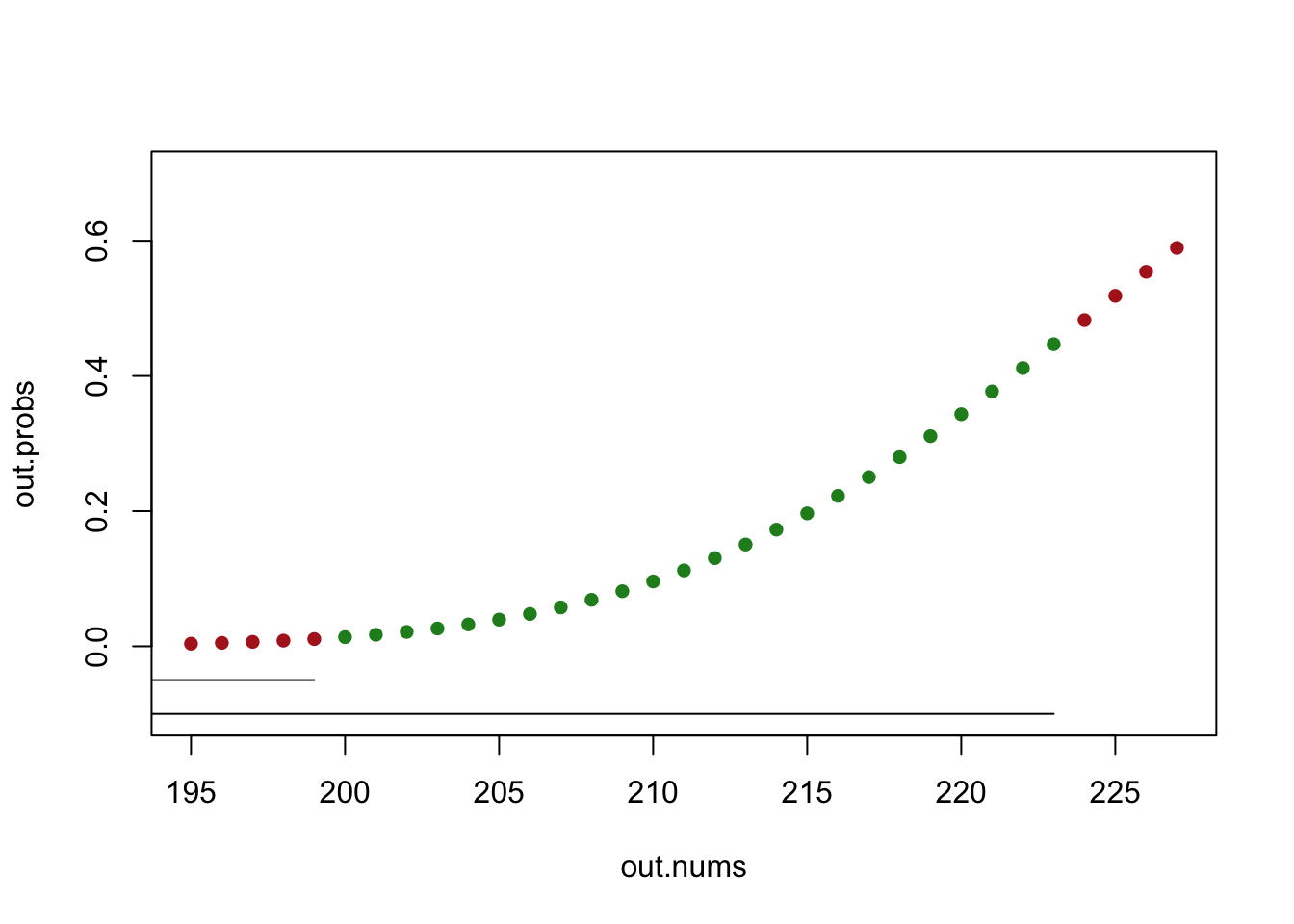
\(Q \sim U(min=10, max=200)\)
(10+200)/2[1] 105((200-10)^2)/12[1] 3008.333dunif(12, min=10, max=200)[1] 0.005263158This gives an answer because it is the graphing value of the PDF at this value, but the correct answer is 0, because the probability of any specific value of a continuous RV is 0.
punif(20, 10,200) - punif(12, 10,200)[1] 0.04210526Trick question! Same answer. Because the probability of being exactly equal is zero this doesn’t change the way we calculate this at all.
punif(20, 10,200) - punif(12, 10,200)[1] 0.04210526\(X \sim N(\mu=26, \sigma^2=49)\)
pnorm(30,26,7, lower.tail=F)[1] 0.2838546pnorm(30, 26, 7) - pnorm(24, 26, 7)[1] 0.3285969qnorm(.75, 26,7)[1] 30.72143.925-.075[1] 0.85qnorm(.075, 26,7)[1] 15.92328qnorm(.925, 26,7)[1] 36.07672#What probability is less than 45 in this normal distribution?
pnorm(45, 26,7)[1] 0.9966791#For the standard normal, what puts that amount of probability in the left tail?
qnorm(pnorm(45, 26,7))[1] 2.714286Here are two tables you would find in the back of a stats textbook.
A Standard Normal (Z) Table (analogous to the pnorm function)
An Inverse Z Table (analogous to the qnorm function)
Answer the following question using these tables and without using R (you can use it as a calculator but can’t use the norm functions).
(a) Women’s height is normally distributed with mean of 64 and a standard deviation of 3. What is the approximate probability a woman has a height between 63 and 66 inches? In a few sentences describe how you got your answer.
How many SD’s above and below the mean are those two points?
(63-64)/3[1] -0.3333333(66-64)/3[1] 0.6666667After finding these two points I can use the linked Z table to look up the probability to the left of those two points in the standard normal distribution. Using the table I find that to the left of -.33 (which is .33 standard deviations below the mean for any normal distribution) is a probability mass of .37. Similarly, using the table I find that to the left of .67 (which is .67 standard deviations above the mean for any normal distribution) is .75 probability mass. As such the probability between these two points is: \(.75-.37=.38=38\%\). 38% of the probability mass is between .33 standard deviations below the mean and .67 standard deviations above the mean. Put back into the terms of the original question: approximately 38% of women are between 63 and 66 inches tall. (Your answer will be around here depending on rounding.)
(b) What height does a woman have to be such that only 2.5% of women are taller than her?
If a woman is shorter than 2.5% of women it means that she is taller than 97.5% of women. Using the inverse z table I can see that the z score that puts 97.5% in the left tail is 1.960.
How many standard deviations away from the mean is that?
64 + (3*1.960)[1] 69.88A woman has to be 69.88 inches tall to be shorter than only 2.5% of women.
(a) month.pmf is a PMF of a random variable representing the probability that you are born in each month of the year, where January is month 1, February is month 2 etc. Using the equations discussed in class, mathematically determine the expected value and variance of this random variable.
month.pmf <- rio::import("https://github.com/marctrussler/IIS-Data/raw/refs/heads/main/MTQ1A.Rds", trust=T)The expected value of a random variable is \(E[X]=\sum xP(x)\). As such, I multiply the number of the month by the probability of that month occurring. The variance is given by \(V[X]=E[X^2] - E[X]^2\). As such I find the expected value of the random variable squared, and subtract off the square of the random variable.
#Expected Value
exp <- sum(month.pmf$month * month.pmf$prob.month)
exp
[1] 6.513661#Variance
var <- sum((month.pmf$month^2) *month.pmf$prob.month) - exp^2
var[1] 11.91102(b) On December 1, 1969 a lottery was held to determine which American men would be drafted to fight in the Vietnam War. All birthdays (including leap day, February 29th) were placed in a large bin and selected one at a time and the order was recorded. The first birthday drawn was September 1st, so men born on September 1st between 1944 and 1950 were the first drafted. The second birthday drawn was April 24th, so men born on that day between 1944 and 1950 were the second group drafted. Ultimately, men from the first 195 numbers drawn were drafted for the war.
The file “VietnamDraft.Rds” contains the actual results of the 1969 draft.
vietnam.draft <- rio::import("https://github.com/marctrussler/IIS-Data/raw/refs/heads/main/MTQ1B.Rds", trust=T)
head(vietnam.draft)
month day drafted
1 1 1 FALSE
2 1 2 TRUE
3 1 3 FALSE
4 1 4 FALSE
5 1 5 TRUE
6 1 6 FALSEIn the data month and day describes each day in the year. drafted is a boolean variable that tells you if people born on a particular day were drafted, or not.
Using these data and the conditional probability formula, determine \(P(M=12 | Drafted=T)\): the probability of having a December birthday conditional on being drafted. Compare this to the unconditional probability of \(P(M=12)\) (the probability of having a December birthday contained in month.pmf). Based on this: is being born in December and being drafted independent events?
#Conditional probability is P(A|B) = P(A&B)/P(B)
mean(vietnam.draft$month==12 & vietnam.draft$drafted)/mean(vietnam.draft$drafted)
[1] 0.1333333#The conditional probability is 13%
month.pmf$prob.month[12][1] 0.08469945#The unconditional probability is 8%The probability of having a December birthday conditional on being drafted is much higher compared to the unconditional probability of being born in December. If these two events were independent then the conditional probability would be equal to the unconditional probability. These two events are not independent.
(c) Maybe the difference you found in (b) was just due to random chance. We can perform a simulation of a “fair” draft by drawing a sample of size 195 from the random variable month.pmf using the sample command. (i.e. we want to draw 195 birthdays that would be selected in the draft. We just care about what month people were born in, so we are going to draw, say, 12 December birthdays, and 8 April birthdays, 9 May birthdays, etc.)
Use the sample command and a for() loop to simulate a fair draft 1000 times. In each of these simulations, determine the proportion of draft days that are in December. The result should be a vector of length 1000 where each entry is the probability of being born in December conditional on being drafted. Compare the distribution of these simulations to the conditional probability from the real draft you calculated in (b). Describe what you see, and what it means in real-world terms.
set.seed(19140)
result <- rep(NA, 1000)

for(i in 1:1000){
draft <- sample(month.pmf$month, 195, prob=month.pmf$prob.month, replace=T)
result[i] <- mean(draft==12)
}

plot(density(result), main="Distribution of P(Dec|Draft) in Fair Draft")
abline(v=mean(vietnam.draft$month==12 & vietnam.draft$drafted)/mean(vietnam.draft$drafted), lty=2, col="firebrick")
legend("topleft", "Observed P(Dec|Draft)", lty=2, col="firebrick")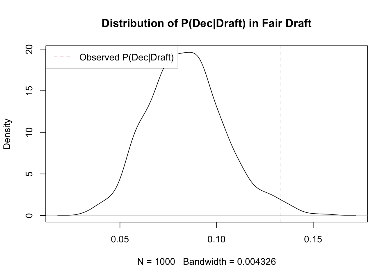
The distribution of fair drafts shows that December birthdays are selected between 0 and 15 percent of the time, though most of the selections are around 8 percent. It is very rare to get a result as extreme as 13%. This suggests that the real-world result was not drawn from this random variable.
In real terms the 1969 Vietnam Draft did not select random birth dates successfully. While not every draftee ultimately served in Vietnam, this error had tragic consequences for those selected, particularly if you consider that draftees were more likely to die in the war compared to enlisted men. You can read more about what happened here. The draft procedure was changed substantially in subsequent years and led to a more random selection.
(d) Calculate \(P(M=m|Drafted=T)\) for each month, and add those points to the below graph to determine if the issues with the draft were limited to December.
plot(month.pmf$month,month.pmf$prob.month, col="darkblue", pch=16, ylim=c(.05,.15), xlab="Month",
     ylab="Probability", main="Comparison of PMFs")
#points(month.pmf$month, YOUR_RESULT,col="firebrick", pch=16)
legend("topleft", c("P(Born in Month)", "P(Born in Month | Selected for Draft)"), pch=c(16,16),
       col=c("darkblue", "firebrick"))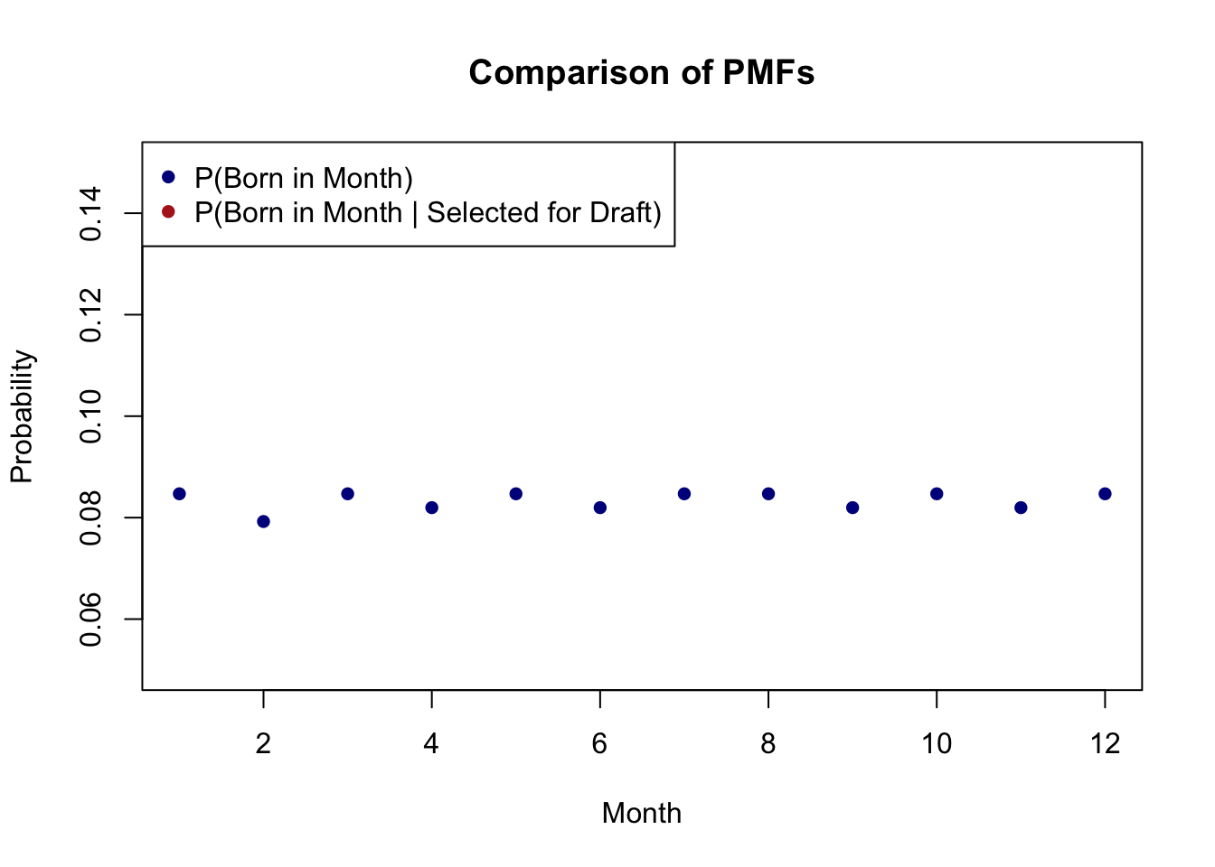
months <- unique(vietnam.draft$month)
prob.selected <- rep(NA, length(months))
for(i in 1:length(months)){
  prob.selected[i] <- mean(vietnam.draft$month==months[i] & vietnam.draft$drafted)/mean(vietnam.draft$drafted)
}

plot(month.pmf$month,month.pmf$prob.month, col="darkblue", pch=16, ylim=c(.05,.15), xlab="Month",
     ylab="Probability", main="Comparison of PMFs")
points(month.pmf$month,prob.selected,col="firebrick", pch=16)
legend("topleft", c("P(Born in Month)", "P(Born in Month | Selected for Draft)"), pch=c(16,16),
       col=c("darkblue", "firebrick"))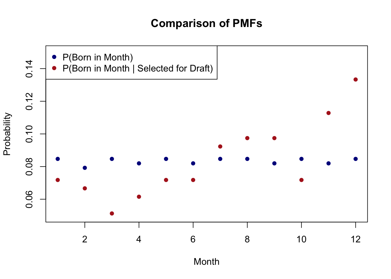
The red dots look very different from the blue dots. The probability of being born in a month early in the year conditional on being drafted is much lower than the unconditional probability of being born in one of those months. On the other hand, the probability of being born late in the year conditional on being drafted is much higher than the unconditional probability of being born in these months. It seems unlikely that the blue random variable could create the red dots.