Problem Set Due Wednesday October 28 at 7pm on Canvas.
You will hand in a .Rmd file and a knitted html output.
I have provided the raw RMD of this problem set you can use as a template for answering.
Question 1
When you show up to a bus stop without checking the schedule, your waiting time can be thought of as a uniform random variable. Suppose buses to campus arrive exactly every 60 minutes, and you arrive at the stop at a completely random moment. Your waiting time \(X\), measured in minutes, is then uniformly distributed between 0 and 60.
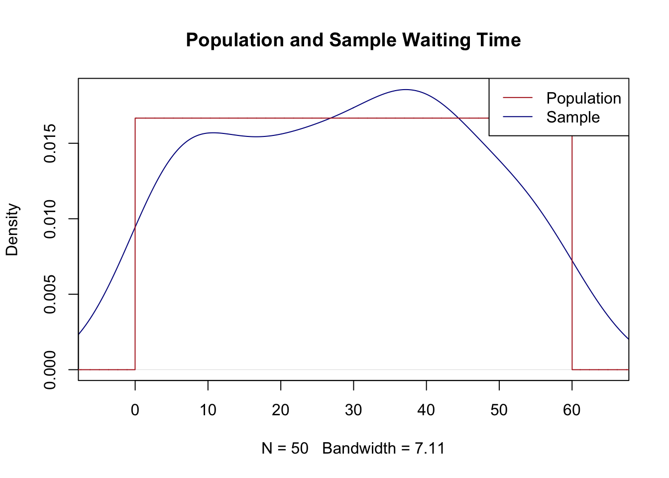
Take a random sample of 50 waiting times. Plot the distribution of the population and your sample of 50. How close are they? Is that what you expected?
set.seed(19104)x <-runif(50, min =0, max =60)mean(x)
[1] 29.19373
var(x)
[1] 298.4041
#The population is Uniform(0,60): a flat density of height 1/60 between 0 and 60.plot(density(x), main ="Population and Sample Waiting Time", col ="darkblue",xlim =c(-5, 65))eval <-seq(-10, 70, .01)points(eval, dunif(eval, 0, 60), col ="firebrick", type ="l")legend("topright", c("Population", "Sample"), lty =c(1, 1),col =c("firebrick", "darkblue"))
The sample is roughly flat, in the ballpark of the uniform population, with a mean near 30 and a variance near 300 (the population values are \(\frac{0+60}{2}=30\) and \(\frac{(60-0)^2}{12}=300\)). It is bumpy and ragged rather than perfectly flat, which is exactly what I’d expect with only 50 observations. The density() smoother also lets the sample spill a little past 0 and 60, which is an artifact of the kernel, not real probability out there.
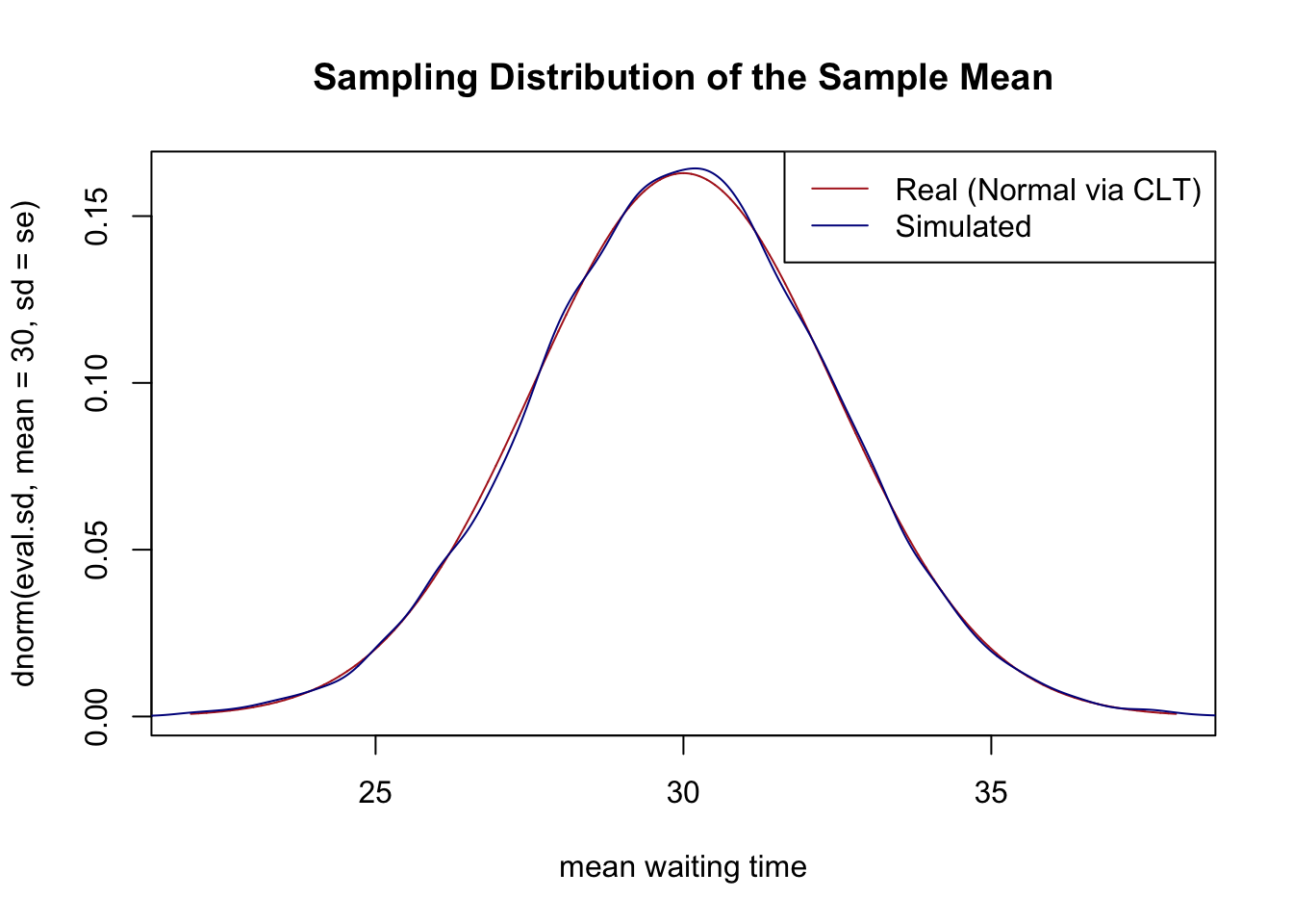
Taking advantage of the fact that I’ve given you information about the population, plot the sampling distribution of the sample mean for \(n=50\). Confirm that this sampling distribution is correct by repeatedly sampling from this population, taking means, and plotting the density of those simulated means. The population is flat and looks nothing like a bell: what shape does the sampling distribution take, and why?
Via the Central Limit Theorem the sampling distribution is \(\bar{X_n}\sim N(\mu=30, \sigma=\frac{sd_x}{\sqrt{n}})\), where the population standard deviation is \(sd_x=\frac{60-0}{\sqrt{12}}\approx 17.32\).
#Standard error, using the known population sd of a Uniform(0,60)se <- (60/sqrt(12)) /sqrt(50)se
[1] 2.44949
#Draw simulated samples and take their meansmeans <-rep(NA, 10000)for(i in1:10000){ means[i] <-mean(runif(50, 0, 60))}#Plot the CLT normal against the simulated meanseval.sd <-seq(22, 38, .001)plot(eval.sd, dnorm(eval.sd, mean =30, sd = se), type ="l", col ="firebrick",main ="Sampling Distribution of the Sample Mean", xlab ="mean waiting time")points(density(means), col ="darkblue", type ="l")legend("topright", c("Real (Normal via CLT)", "Simulated"), lty =c(1, 1),col =c("firebrick", "darkblue"))
The sampling distribution is a normal distribution (a bell), centered at 30 with a standard error of about 2.45, even though the population it is built from is perfectly flat. This is the Central Limit Theorem at work: the distribution of the mean is normal regardless of the shape of the population it is drawn from. The simulated means line up almost perfectly with the theoretical normal.
Calculate the probability that the mean waiting time in a sample of 50 people will be less than 28 minutes. Confirm your answer with the simulated results from (b).
#Calculated, using the sampling distribution N(30, se)pnorm(28, mean =30, sd = se)
[1] 0.2071081
#From simulationmean(means <28)
[1] 0.2022
#Effectively the same.
About 0.21.
Calculate the probability that the mean waiting time in a sample of 50 people will be between 28 and 32 minutes. Confirm your answer with the simulated results from (b).
#Calculatedpnorm(32, 30, se) -pnorm(28, 30, se)
[1] 0.5857838
#From simulationmean(means >28& means <32)
[1] 0.5921
#Again, effectively the same.
About 0.59.
What is the probability that a single person waits less than 28 minutes? What is the probability that a single person waits between 28 and 32 minutes? Give the answers, and then say in words why these answers are not the same as the answers for (c) and (d).
#A single person comes from the POPULATION (the flat uniform), not the#sampling distribution of the mean.punif(28, 0, 60)
[1] 0.4666667
punif(32, 0, 60) -punif(28, 0, 60)
[1] 0.06666667
For a single person the answers are about 0.47 and 0.07. These are different from (c) and (d) because they ask about the population, not the sampling distribution of the mean. A single waiting time is uniform: it can land anywhere from 0 to 60 with equal density, so it is quite likely to be below 28 (0.47) and quite unlikely to fall in a narrow 4-minute band (0.07). The mean of 50 waits, by contrast, is squeezed into a narrow normal distribution around 30, so it is less likely to be as low as 28 (0.21) and much more likely to sit in that same 4-minute band around the center (0.59). Averaging many draws kills off the variation that a single draw still has.
What size \(n\) would you need to be 99% certain that the mean waiting time in a sample will be between 28 and 32 minutes? Determine this answer and then repeatedly sample from the population with a sample of that size to show that 99% of sample means do indeed fall within those bounds.
We want the \(n\) that makes us 99% certain the sample mean is within 2 minutes of the truth (30). The value of the standard normal that puts 99% of the probability mass in the center is 2.576. We need the standard error to be small enough that 2 minutes represents 2.576 standard errors:
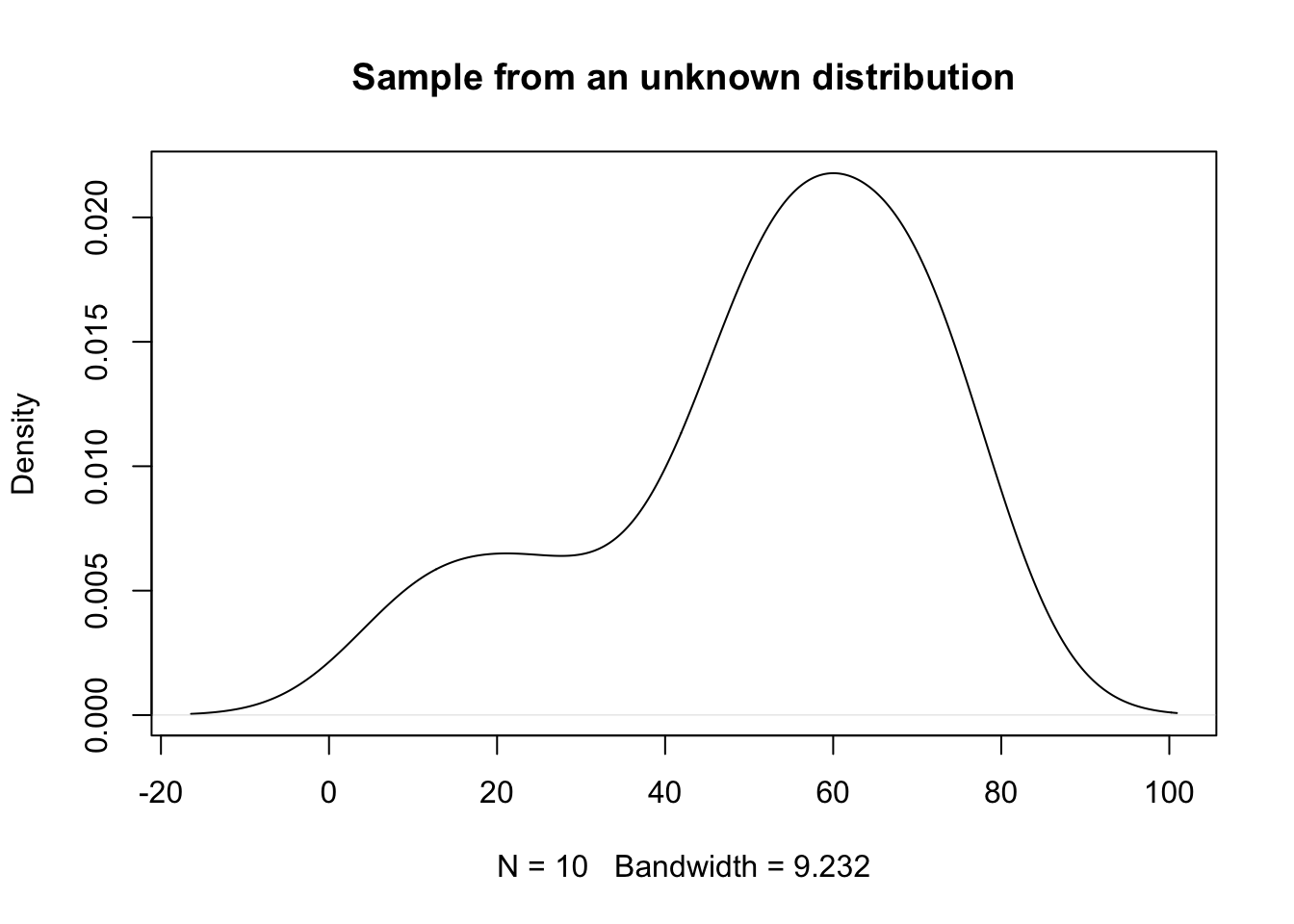
Plot the distribution of this sample and determine the mean and variance. Using your intuition: what do you expect the distribution that produced this sample might have looked like? (Ignore that I tell you more below, genuinely try to think about how you would answer this question if you didn’t know.)
mean(x)
[1] 51.75393
var(x)
[1] 403.601
sd(x)
[1] 20.08982
plot(density(x), main ="Sample from an unknown distribution")
The sample mean is about 51.8 and the sample standard deviation is about 20. With only 10 observations it is genuinely hard to say much about the shape: it could be normal, though it looks a little lumpy. I would guess the true mean is somewhere in the 40s or 50s, but with this little data I would not be confident about much more than that.
(Again ignoring that I tell you the population that this sample is drawn from below) Using only information contained in this one sample produce a 70%, 90% and 95% confidence interval around the mean of this sample. For each, describe in words what the confidence interval is telling you.
Because we only have 10 observations and are estimating the standard deviation from the sample itself, we take our critical values from the \(t\)-distribution with \(n-1=9\) degrees of freedom, not the normal.
#Standard errorse <-sd(x) /sqrt(10)#70%t <-qt(.15, df =9) *-1c(mean(x) - se * t, mean(x) + se * t)
[1] 44.76747 58.74038
#About [44.8, 58.7].#90%t <-qt(.05, df =9) *-1c(mean(x) - se * t, mean(x) + se * t)
[1] 40.10823 63.39962
#About [40.1, 63.4].#95%t <-qt(.025, df =9) *-1c(mean(x) - se * t, mean(x) + se * t)
[1] 37.38253 66.12532
#About [37.4, 66.1].
The 95% interval is the widest and the 70% the narrowest: the more confident we want to be that the interval captures the truth, the wider we have to cast the net. The correct language is that “X% of similarly constructed confidence intervals will contain the true population mean.” Notice that 56 sits comfortably inside all three intervals.
A colleague claims the true population mean is 56. Without using the t.test() function, carry out the five-step hypothesis test of \(H_0: \mu = 56\) against \(H_1: \mu \neq 56\) (a two-tailed test). Do this at three significance levels: \(\alpha = .30\), \(\alpha = .10\), and \(\alpha = .05\). For each \(\alpha\) report the result of the hypothesis test. Then confirm that your decision at each \(\alpha\) is the same as what you would conclude from the confidence intervals in (b).
We run the five steps once; the test statistic and p-value don’t change with \(\alpha\), only the comparison in step 5 does.
1. Specify a null and alternative hypothesis.\(H_0: \mu = 56\) against \(H_a: \mu \neq 56\) (a two-tailed test).
2. Choose a test statistic and \(\alpha\). The test statistic is the sample mean, and we will run the test at \(\alpha = .30\), \(.10\), and \(.05\).
mean(x)
[1] 51.75393
3. Derive the sampling distribution. Under the null the sampling distribution of the mean is \(t\) distributed with \(n-1 = 9\) degrees of freedom, centered on 56. Its standard error is:
se <-sd(x) /sqrt(10)se
[1] 6.35296
4. Compute the p-value. First, how many standard errors is our test statistic from the null, and then the two-tailed area beyond that in the \(t\)-distribution with 9 degrees of freedom:
t.score <- (mean(x) -56) / set.score
[1] -0.6683616
2*pt(abs(t.score), df =9, lower.tail =FALSE)
[1] 0.5206738
5. Reject or retain the null. The p-value is about 0.52. That is greater than .30, .10, and .05, so at all three levels we fail to reject\(H_0: \mu = 56\).
This lines up exactly with the confidence intervals in (b): 56 sits inside the 70%, 90%, and 95% intervals, so at none of these levels can we rule it out. The confidence interval and the hypothesis test are two views of the same thing.
Confirm your test statistics and p-values using t.test(x, mu = 56, conf.level = xx).
t.test(x, mu =56, conf.level = .70)
    One Sample t-test

data:  x
t = -0.66836, df = 9, p-value = 0.5207
alternative hypothesis: true mean is not equal to 56
70 percent confidence interval:
 44.76747 58.74038
sample estimates:
mean of x
 51.75393
t.test(x, mu =56, conf.level = .90)
    One Sample t-test

data:  x
t = -0.66836, df = 9, p-value = 0.5207
alternative hypothesis: true mean is not equal to 56
90 percent confidence interval:
 40.10823 63.39962
sample estimates:
mean of x
 51.75393
t.test(x, mu =56, conf.level = .95)
    One Sample t-test

data:  x
t = -0.66836, df = 9, p-value = 0.5207
alternative hypothesis: true mean is not equal to 56
95 percent confidence interval:
 37.38253 66.12532
sample estimates:
mean of x
 51.75393
Every call reports the same test statistic (\(t = -0.67\)) and p-value (\(0.52\)), confirming the hand calculation in (c). The confidence interval printed by each call matches the matching interval from (b), which is the duality again: t.test hands you the test and the interval together.
This sample was produced by rnorm(10,56,32) (the true mean is, indeed, 56). Write a loop that repeatedly (i) draws a fresh sample of 10 from this population, (ii) builds 70%, 90% and 95% confidence intervals, and (iii) runs your \(\alpha = .30/.10/.05\) test of \(H_0: \mu = 56\). Across many repetitions, show two things: that roughly 70%, 90% and 95% of the intervals contain 56, and that your tests land in the rejection region (reject \(H_0\)) roughly 30%, 10% and 5% of the time. Explain why “the percent of intervals that miss 56” and “the percent of tests that reject” are the same number, and why that number is \(\alpha\).
set.seed(19104)reps <-10000levels <-c(.70, .90, .95)alphas <-1- levels #.30, .10, .05contains <-matrix(NA, reps, 3) #does the CI contain 56?reject <-matrix(NA, reps, 3) #does the test reject 56?for(i in1:reps){ xs <-rnorm(10, 56, 32) se <-sd(xs) /sqrt(10) t.score <- (mean(xs) -56) / se#Two-tailed p-value, using the absolute t so it works whether the sample#mean landed above or below 56. p <-2*pt(abs(t.score), df =9, lower.tail =FALSE)for(j in1:3){ tcrit <-qt(1- alphas[j] /2, df =9) ci <-mean(xs) +c(-1, 1) * tcrit * se contains[i, j] <- ci[1] <=56& ci[2] >=56 reject[i, j] <- p < alphas[j] }}#Coverage: should be about .70, .90, .95colMeans(contains)
[1] 0.7072 0.9085 0.9549
#Rejection rate: should be about .30, .10, .05colMeans(reject)
[1] 0.2928 0.0915 0.0451
The intervals contain 56 right around 70%, 90%, and 95% of the time, and the tests reject right around 30%, 10%, and 5% of the time.
These two numbers are not just close, they are identical in every single repetition: reject is always the exact opposite of contains. That is because the \((1-\alpha)\) confidence interval is, by construction, the set of null values we would not reject at level \(\alpha\). So “56 falls outside the interval” and “the test rejects 56” are literally the same event, and their long-run percentages have to match.
And why is that percentage \(\alpha\)? Because here the null is actually true (the real mean is 56). Every time we reject, we are making a false positive, and the whole point of \(\alpha\) is that it sets the rate at which a correct null gets wrongly rejected. So a test run at \(\alpha\) against a true null rejects \(\alpha\) of the time, which is the same as saying a \((1-\alpha)\) interval misses the truth \(\alpha\) of the time.
(One caveat worth noticing: these rates only line up at \(n = 10\) because we used the \(t\)-distribution. If we had used the normal, the intervals would be a touch too narrow, coverage would fall short of 70/90/95, and the tests would reject a bit too often. That is the small-sample correction the \(t\)-distribution exists to make.)