plot(0:14,dbinom(0:14, 14, prob=.1), pch=16, xlab="Number of Left Handed People", ylab="Probability")
Like the class handouts, this review is meant to be a supplement to the textbook, not a replacement. Studying solely from this review will not be sufficient preparation for the midterm.
So far in this class we have covered the basics of probability theory, random variables, principles of sampling, and the standard error of the mean.
What was the point of all this? What’s the big picture?
We started the class talking though the relationship between samples and the population. The population is an unknowable thing, and we want to use a singular sample of data to make inferences about that population. On first blush that seems impossible. I get a survey of 5000 people where 43% support the President…. what can I possibly say about every American?
Our journey through probability helped us to re-frame that question.
Critically, we learned how we can use the rules and axioms of probability to model variation due to random chance. Specifically, we learned the rules of probability to help us to generate random variables, which are descriptions of various events that can happen with attached probabilities. Once we understand the potential variation due to random chance we can assess the likelihood of observing our data given an assumption about the population.
For example, we looked at what the expected number of left handed people would be for 14 people:
plot(0:14,dbinom(0:14, 14, prob=.1), pch=16, xlab="Number of Left Handed People", ylab="Probability")
We compared this probability to our observation that 6/14 people were left handed. In this case the probability of that occurring due to random chance was very low. We may decide to reject that this distribution is what is generating Presidents.
To do a more relevant example: The Atlanta Braves, who won 64.2% of their games in the regular season just lost 3/4 games to the Philadelphia Phillies in the National League Division Series. Certainly this will lead to all sorts of re-working and re-toolings of their franchise. But what is likely to occur by random chance to a team that wins 64.2% of their games over the course of 4 games:
dbinom(0:4, 4, .642)[1] 0.01642601 0.11782680 0.31694752 0.37892050 0.169879161.6% of the time they win no games, and 11.7% they win only 1 game (what happened). This is, by no means, a rare outcome! Things that happen 10% of the time happen all the time. The Braves were just unlucky (but are also trash and deserved to lose to our Fightin’ Phils).
All of this requires us to know the shape of the random variable in the population. That’s easy for things like the binomial distribution. It was more difficult when we started to think about having a singular mean and not knowing the random variable which produced it.
Through the LLN and CLT we discovered that the sampling distribution of the sample mean (the random variable which produces means) is a very predictable thing. Because of this, we can go through a similar process of observing a sample, postulating something about the population, and then determining the likelihood of our sample given that postulate.
If I was to sum up what we’ve learned so far in a few sentences I would say:
Populations/Data Generating Processes are unknowable. The best we can do is to make an assumption about the population, use our knowledge of random variables to model the uncertainty and range of possibilities that assumption would generate, and then estimate the likelihood that assumption is true given our sample of data.
The following goes section by section, highlighting some of the key lessons from each.
Probability denotes the expected long-term frequency of events. A definition that I find helpful:
The chance of something gives the percentage of time it is expected to happen, when the basic process is done over and over again, independently and under the same conditions.
To formalize our look into probability, two key terms are events and a sample space. Events are simply outcomes of a particular thing: the outcome of the roll of a dice or a flip of a coin; or the outcome of a presidential election; or whether a randomly sampled individual is favorable towards the President or not. A sample space is set of all possible outcomes of the thing we are considering.
When probability of all events is equal we can then define the probability of an event occurring by dividing the number of elements in the event by the total number of outcomes in the sample space.
There are a couple of “rules” (axioms) about probability that are helpful to keep in mind.
The probability of any event A is non-negative: \(P(A)\geq 0\).
The probability that one of the outcomes in the sample space occurs is 1. \(P(\Omega)=1\)
\(P(AorB) = P(A) + P(B) - P(A\&B)\) (What does this reduce to if A and B are mutually exclusive?)
Basic simulation of a roll of the dice:
set.seed(19104)
dice <- c(1,2,3,4,5,6)
result <- rep(NA,10000)
  for(i in 1:10000){
    result[i] <- sample(dice,1,replace=T)
  }
table(result)
result
1 2 3 4 5 6
1684 1653 1710 1682 1676 1595 We know that each number of a fair dice will come up 1/6 of the time, so our expectation would be that each of these numbers would be drawn \(10000/6=1666\) times. Obviously with random chance we don’t get that number exactly, but each is quite close.
Permutations are sequences where the order matters. The formula is \(_nP_k = \frac{n!}{(n-k)!}\), which gives the number of permutations where \(n\) is the number of options and \(k\) is the number of selections.
A combination differs from a permutation because with a combination the order does not matter. A lottery is a great example of this. You win the lottery if the numbers you selected come out of the bin, regardless of the order of the balls. The formula is \(_nC_k = \frac{n!}{k!(n-k)!}\).
What is the difference between these two (mathematically, and what does it do?)
Calculating combinations in R:
choose(70,5)[1] 12103014Calculating permutations in R (why does this work?):
(choose(365,20)*factorial(20))[1] 1.036691e+51Conditional probability is about sub-setting. If we are theoretically interested in P(A|B=b), we want to think about sub-setting to the cases for B where that’s true, and recalculating the probability of A with that new denominator.
The formula for a conditional probability is \(P(A|B) = \frac{P(A\&B)}{P(B)}\).
Two events are independent if:
\[ \begin{aligned} P(A|B)=P(A)\\ \& \\ P(B|A)=P(B) \end{aligned} \]
All of the probability up to this point has assumed equal probability between events. We have also mostly dealt with things that were fairly countable.
We used the example of determining if Mahomes’ performance in the Super Bowl would be particular or not, with the background that he had a certain known success rate (say 63%) and could throw any number of passes (20,21,22,23….). We want to be able to determine for any combination of success rates and attempts what the probability was of all number of successes.
To determine this we derived the binomial formula:
\[ P(K=k) = {_nC_k} * \pi^k *(1-\pi)^{n-k} \]
The first part tells us the number of ways to have k successes in n trials. The second part tells us, for each of those ways to have k successes, what the probability is.
To get the second part we also derived that when two events are independent:
\[ \begin{aligned} P(A|B) = \frac{P(A\&B)}{P(B)}\\ P(A|B) = P(A) \; \text{iff} \perp\\ \therefore P(A) = \frac{P(A\&B)}{P(B)}\\ P(A\&B) = P(A) * P(B) \; \text{iff} \perp \end{aligned} \]
We moved on from there to formally define a RV: When we talk about “random variables” this is a different thing than the variables in a dataset (which are samples of data). When we talk about random variables we are talking about population level distributions that produce sample of data, with each of those samples being a little bit different, yet following the same underlying truth.
In short, Random Variables are helpful because they allow us to compare a sample of data to the theoretical truth of what should happen. In other words, we can compare a sample of data to the population.
Formally, a random variable assigns a number and a probability to each event. Because we are defining events with a number and a probability, this allows us to do math! Which is good!
The probability mass function and cumulative distribution function are complements of one another. With one you can derive the other.
So for this PMF
\[ f(x) = P(C=c) = \begin{cases} .1 \text{ if } 0 \\ .25 \text{ if } 1 \\ .5 \text{ if } 2 \\ .15 \text { if } 3 \\ \end{cases} \]
We can derive this CDF:
\[ F(x) = P(C \leq c) = \begin{cases} 0 \text{ if } < 0\\ .1 \text{ if } \geq 0 \& < 1 \\ .35 \text{ if } \geq 1 \& <2 \\ .85 \text{ if } \geq 2 \& < 3 \\ 1 \text { if } \geq 3 \\ \end{cases} \]
For any random variable we can describe the expectation and variance. These are population features of random variables and do not apply to samples of data.
The expected value of a random variable is: \(E[X] = \sum_x xp(x)\)
The variance of a random variable is: \(V[X] = E[(X-E(X))^2]\) or \(V[X] = E(X^2) - E(X)^2\)
A Bernoulli RV describes a single success or failure. It has one parameter, \(\pi\) the probability of success. The expected value is \(\pi\) and the variance is \(\pi*(1-\pi)\). What is an example of a Bernoulli RV?
A binomial RV describes a sequence of Bernoulli RVs. It has two parameters. \(\pi\) the probability of success of each Bernoulli, and \(n\), the number of Bernoulli draws. The expected value is \(n*\pi\) and the variance is \(n*\pi*(1-\pi)\). What is an example of a Binomial RV?
A continuous RV can take on an infinite number of values within a given interval. As such, the probability of a continuous RV taking on any particular value is 0, as if it was anything greater than 0 then the CDF would not approach 1, but infinity.
Instead of Probability Mass Functions, continuous variables have Probability Density Functions, which give the probability for a range of values. To get a CDF from a PDF we integrate from negative infinity to any given value. To get a PDF from a CDF we take the derivative at any given value.
The first important continuous distribution we considered was the uniform distribution, which takes on an equal probability within a given interval defined by end-points \(a\) and \(b\). The PDF of a uniform RV is given by:
\[ f(X) = \begin{cases} \frac{1}{b-a} \text{ if } a \leq x \leq b\\ 0 \text{ otherwise} \end{cases} \]
The expected value of a uniform RV is given by: \(E[X] = \int_a^b x*f(x) \partial x = \text{Math!} = \frac{a+b}{2}\).
The variance of a uniform RV is given by: \(V[X] = E[X^2] - E[X]^2 = \text{Math!} = \frac{1}{12}(b-a)^2\).
The normal random variable is the most important random variable. It has two parameters: \(\mu\) the central tendency of the distribution, and \(\sigma\) the standard deviation of the distribution. The normal distribution is always symmetrical. The PDF of the normal distribution is defined by:
\[ f(x) = \frac{1}{\sqrt{2\pi \sigma^2}} e^{- \frac{1}{2\sigma^2}(x-\mu)^2} \]
But given this if we have a \(\mu\) and a \(\sigma\) we can conclude anything we want about the normal distribution.
We discussed how the properties of the normal distribution meant that if we make the following translation to any normal distribution:
\[ Z = \frac{X-\mu}{\sigma} \]
We are left with the standard normal distribution: \(Z \sim N(0,1)\).
The standard normal distribution is helpful because it allows us to talk about normal distribution in “standard deviation units”. If you tell me that 2.57 units in the standard normal contains 99% of all probability mass, that means that 2.57 standard deviations from the mean contains 99% of the probability mass in all normal distributions.
We learned that we can use R to calculate various probabilities and values for known random variables using built in functions. The key thing here is that we have already worked out the shape of these probability distributions, and if you know the parameters to define them, R can give you a large number of answers. See notes!
One helpful shortcut I covered but want to highlight: keep in mind that these functions can take whole vectors of information.
So if I had 4 normal distributions with \(\mu = \lbrace 2,4,3,6 \rbrace\) and \(\sigma = \lbrace 1,1.2,1.3,1.8\rbrace\) and I wanted to know what value for each of them put 40% probability in the left tail, I could do them all separately:
qnorm(.4,2,1)[1] 1.746653qnorm(.4,4,1.2)[1] 3.695983qnorm(.4,3,1.3)[1] 2.670649qnorm(.4,6,1.8)[1] 5.543975Or I could put that information in vectors and do it all at once:
mu = c(2,4,3,6)
sigma = c(1,1.2,1.3,1.8)

qnorm(.4,mu, sigma)
[1] 1.746653 3.695983 2.670649 5.543975Think about the potentials for this so scale up.
The probability distribution random variables discussed thus far were populations that we could sample from. We did not, at this point have tools to determine how good of a sample we will have when we increase the sample size from 1 to 2 to 3…. to infinity.
We learned three key principles of sampling:
To be clear: these are principles which are about the sample mean specifically, but will eventually apply to all estimates that we form from a sample.
Critically: the sample mean itself is drawn from a random variable with a known shape (above). That distribution is the sampling distribution, and the standard deviation of that sampling distribution is the standard error. Because that shape is known we can project with a great deal of confidence what a large number of sample means will look like if we understand the distribution from which they are being pulled.
To be clear about the above: X is any distribution. It could be binomial, Bernoulli, uniform, normal, totally crazy. It doesn’t matter. But if we know the expected value and variance of those distributions, then we can project with confidence what estimated sample means from those distributions will look like.
Population parameters are true, fixed, values. We use an estimator (a method) to produce an estimate (a single number in our sample) which is one of an infinite number of estimates that can be drawn from an infinite number of samples.
An estimator is unbiased if:
\[ E[estimate-truth]=0 \]
We can determine unbiasedness through sampling, but also through mathematical proof.
For the latter, we wish to know whether:
\[ E[\phi] -E[X]=0 \] Where \(\phi\) is any estimator.
The key features of the expectation operator were that:
\[ E[cX] = c*E[X] \]
Where \(c\) is a constant.
\[ E[X_1] = E[X] \]
The expected value of any observation is equal to the overall expected value of the random variable.
More than unbiasedness, we want our estimators to be consistent, which is when they are unbiased and the variance of the estimator gets smaller as \(n\) increases.
We can take the variance of our estimator to determine this through mathematical proof.
For the variance estimator:
\[ V[cX] = c^2*V[X] \]
If we take a constant out of the variance operator it gets squared.
\[ V[X_1]=V[X] \] The variance of any given observation is also equal to the overall variance of the random variable.
We can measure if the estimator is consistent by whether the MSE/RMSE goes to 0 when sample size goes to infinity, where MSE:
\[ MSE = Variance +Bias^2 = V[\hat{\theta}] + (E[\hat{\theta}- \theta])^2 \]
Everything above about the sampling distribution assumed we knew the population variance \(V[X]\). In the real world we don’t! We only ever have our one sample.
The standard deviation of the sampling distribution of the mean – the standard error – is:
\[ SE[\bar{X}] = \frac{\sigma}{\sqrt{n}} \]
Because we don’t know the population standard deviation \(\sigma\), we estimate it using the sample standard deviation \(s\):
\[ \widehat{SE}[\bar{X}] = \frac{s}{\sqrt{n}} \]
This is the key move that lets us do inference from a single sample: the sample gives us both an estimate of the mean (\(\bar{x}\)) and an estimate of how much that mean would bounce around from sample to sample (\(\widehat{SE}\)). It turns out that using the sample standard deviation/variance as a stand in for the population level variables works good enough. (With the t-distribution caveat listed below).
Subbing in the sample standard deviation solves one problem (what is the shape of the sampling distribution?) but doesn’t solve where the sampling distribution should be. One way to solve this is with a confidence interval, where we center the sampling distribution at the sample mean.
Because the sampling distribution is normal, we know that about some percentage of sample means fall within roughly two standard errors of the truth. Running that logic backwards, we can build an interval around our estimate that will capture the true population mean a percentage of of the time:
\[CI(\alpha) = [\bar{X_n}-z_{\alpha/2}*SE,\bar{X_n}+z_{\alpha/2}*SE]\]
The z-score in that equation will change based on what confidence level you want. For a 95% confidence interval the \(\alpha\) will be .05, and therefore we want the z-score for 0.025 (1.96).
Interpreting this correctly is subtle. It is technically not that there is a 95% chance the truth sits inside our particular interval (though I’m fine with this). The truth is a fixed value, either in our interval or not. The technically correct thing is that “95% of similarly constructed confidence intervals contain the true population paramater”.
There is one wrinkle. When we swap the unknown \(\sigma\) for the sample estimate \(s\), we add a little extra uncertainty, because \(s\) is itself an estimate that varies from sample to sample. To account for this, we take our critical values not from the standard normal (\(Z\)) but from the t-distribution.
The t-distribution looks like the standard normal but with fatter tails, which gives us slightly wider – more honest – intervals. Its exact shape is governed by the degrees of freedom, equal to \(n-1\).
The smaller the sample, the fatter the tails and the bigger the correction. As \(n\) grows, \(s\) becomes a reliable estimate of \(\sigma\), the tails thin out, and the t-distribution converges to the standard normal. For large samples the two are practically identical – which is why the “1.96” from the normal still works as a rule of thumb. That being said, if you are asked to estimate a confidence interval or hypothesis test using the sample standard deviation, you must use the t-distribution to get the probabilities.
This is a question from a previous midterm exam. It’s inappropriate for a hand-written exam, so I’ve included it here. You can find the answers below.
elect contains results from the 2020 presidential election. For each state plus DC I have given the two party percentage won by Biden (i.e. the percentage of the vote won by Biden among those who voted for Biden or Trump). Consider this the true level of support for Biden in each of these states.
elect <- rio::import("https://github.com/marctrussler/IIS-Data/raw/main/ElectionData1801Midterm.Rds", trust=T)
head(elect)
state biden.perc
1 AK 0.4473815
2 AL 0.3708863
3 AR 0.3578757
4 AZ 0.5015683
5 CA 0.6490891
6 CO 0.5693832Consider performing a poll of 500 people in each of these states. In each poll the proportion of voters who support Biden would be calculated (i.e. the mean of the variable telling us whether each person supports Biden over Trump). We know that these means will be drawn from a sampling distribution that is normally distributed and centered on the true population value in each state, which in this case is biden.perc.
(a) Add a new column to the data set which gives, for each state, the standard error of the sampling distribution of the mean. (Hint: the random variable we are sampling – the true level of support for Biden in each state – is a Bernoulli.)
(b) We now have the expected value and variance of the (normally distributed) sampling distribution that proportions will be drawn from in each state. Add a new column to the data set which gives, for each state, the probability that the proportion of Biden’s support from a poll of 500 people will be within 2 percentage points of the true value in that state. For example if the true support for Biden in a state is 52.5%, what is the probability a poll of 500 people will have an estimate of Biden support that is between 50.5% and 54.5%?.
(c) We can use R to simulate polls of voters from these states. For example, for the first state I can draw 1000 polls of 500 people and calculate the Biden percent in each like this:
props <- rbinom(1000,500, prob=elect$biden.perc[1])/500Use the above code and a for() loop to draw 1000 “polls” of 500 voters from each of these states. Each time through the loop (i.e for each state) determine the proportion of simulated polls that are within 2 percentage points of the truth and save that information in a new column in elect. Put this column and what you found in (b) in the graphs below to show that your answer for (b) is correct.
#Replace CALCULATED_PROP and SIMULATED_PROP with the values from (b) and (c)

#plot(elect$CALCULATED_PROP, elect$SIMULATED_PROP, pch=16, xlab="Calculated",
#     ylab="Simulated", main="Probability of Sample Mean within 2pp", type="n")
#text(elect$CALCULATED_PROP, elect$SIMULATED_PROP,elect$state)
#abline(0,1)
#
##Same graph without DC to better see all states:
#
#plot(elect$CALCULATED_PROP, elect$SIMULATED_PROP, pch=16, xlab="Calculated",
#     ylab="Simulated", main="Probability of Sample Mean within 2pp", type="n",
#     ylim=c(.6,.75), xlim=c(.6,.75))
#text(elect$CALCULATED_PROP, elect$SIMULATED_PROP,elect$state)
#abline(0,1)
(d) (Bonus) Add a final column that, in each state, gives the number of respondents (rounded to the nearest whole number) that would ensure that 99% of all estimates of Biden’s support will be within 1 percentage point of the true value. As a first step, calculate the number of standard deviations above and below the mean in the standard normal distribution that contain 99% of the probability mass. Then think about writing an equation where \(n\) is the only unknown and isolating it.
elect contains results from the 2020 presidential election. For each state plus DC I have given the two party percentage won by Biden (i.e. the percentage of the vote won by Biden among those who voted for Biden or Trump). Consider this the true level of support for Biden in each of these states.
elect <- rio::import("https://github.com/marctrussler/IIS-Data/raw/main/ElectionData1801Midterm.Rds", trust=T)
head(elect)
state biden.perc
1 AK 0.4473815
2 AL 0.3708863
3 AR 0.3578757
4 AZ 0.5015683
5 CA 0.6490891
6 CO 0.5693832Consider performing a poll of 500 people in each of these states. In each poll the proportion of voters who support Biden would be calculated (i.e. the mean of the variable telling us whether each person supports Biden over Trump). We know that these means will be drawn from a sampling distribution that is normally distributed and centered on the true population value in each state, which in this case is biden.perc.
(a) Add a new column to the data set which gives, for each state, the standard error of the sampling distribution of the mean. (Hint: the random variable we are sampling – the true level of support for Biden in each state – is a Bernoulli. You have the information you need in each state to determine \(V[X]\).).
First calculate the standard error of the sampling distribution in each state, which is the square root of the variance of the Bernoulli random variable divided by the sample size:
elect$se <- sqrt((elect$biden.perc*(1-elect$biden.perc))/500)
head(elect$se)
[1] 0.02223651 0.02160230 0.02143831 0.02236057 0.02134350 0.02214434(b) We now have the expected value and variance of the (normally distributed) sampling distribution that proportions will be drawn from in each state. Add a new column to the data set which gives, for each state, the probability that the proportion of Biden’s support from a poll of 500 people will be within 2 percentage points of the true value in that state. For example if the true support for Biden in a state is 52.5%, what is the probability a poll of 500 people will have an estimate of Biden support that is between 50.5% and 54.5%?.
To get the proportion of means that will be within 2 percentage points of the truth for each states, for each of the sampling distributions I can subtract the probability that is to the left of \(\mu-.02\) from the probability that is to the left of \(\mu+.02\), leaving just the probability that is in the middle.
elect$prop.within.2 <- pnorm(elect$biden.perc+.02, mean=elect$biden.perc, sd=elect$se) - pnorm(elect$biden.perc-.02, mean=elect$biden.perc, sd=elect$se)
head(elect$prop.within.2)
[1] 0.6315718 0.6454643 0.6491331 0.6289090 0.6512690 0.6335618(c) We can use R to simulate polls of voters from these states. For example, for the first state I can draw 1000 polls of 500 people and calculate the Biden percent in each like this:
props <- rbinom(1000,500, prob=elect$biden.perc[1])/500Use the above code and a for() loop to draw 1000 “polls” of 500 voters from each of these states. Each time through the loop (i.e for each state) determine the proportion of simulated polls that are within 2 percentage points of the truth and save that information in a new column in elect. Put this column and what you found in (b) in the graphs below to show that your answer for (b) is correct.
#Replace CALCULATED_PROP and SIMULATED_PROP with the values from (b) and (c)

#plot(elect$CALCULATED_PROP, elect$SIMULATED_PROP, pch=16, xlab="Calculated",
#     ylab="Simulated", main="Probability of Sample Mean within 2pp", type="n")
#text(elect$CALCULATED_PROP, elect$SIMULATED_PROP,elect$state)
#abline(0,1)
#
##Same graph without DC to better see all states:
#
#plot(elect$CALCULATED_PROP, elect$SIMULATED_PROP, pch=16, xlab="Calculated",
#     ylab="Simulated", main="Probability of Sample Mean within 2pp", type="n",
#     ylim=c(.6,.75), xlim=c(.6,.75))
#text(elect$CALCULATED_PROP, elect$SIMULATED_PROP,elect$state)
#abline(0,1)
Here I loop across state, drawing from a binomial with \(n=500\) and \(\pi=biden.perc_i\) 1000 times. I divide each of those draws by 500 to get the sample proportion in each of the 1000 samples. For those 1000 samples I test how many are within 2% of the true population value.
elect$sim.prop.within.2<- NA

for(i in 1:nrow(elect)){
samp.means <- rbinom(1000,500,prob=elect$biden.perc[i])/500
#Test A
elect$sim.prop.within.2[i] <- mean(samp.means>=(elect$biden.perc[i]-.02) & samp.means<=(elect$biden.perc[i]+.02))
}plot(elect$prop.within.2, elect$sim.prop.within.2, pch=16, xlab="Calculated",
ylab="Simulated", main="Probability of Sample Mean within 2pp", type="n")
text(elect$prop.within.2, elect$sim.prop.within.2,elect$state)
abline(0,1)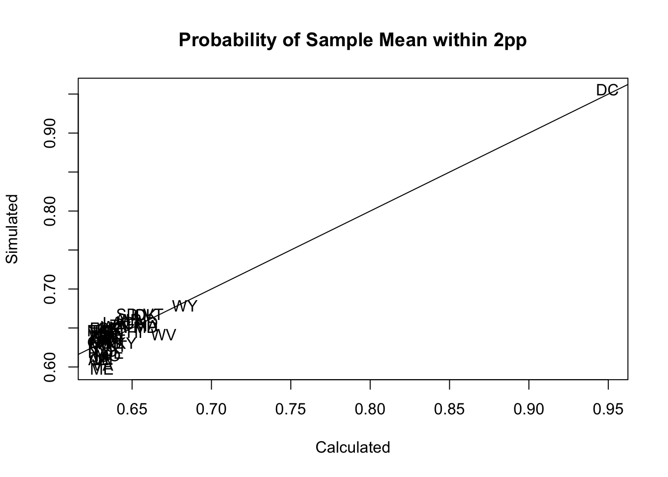
#Without DC to better see all states:

plot(elect$prop.within.2, elect$sim.prop.within.2, pch=16, xlab="Calculated",
     ylab="Simulated", main="Probability of Sample Mean within 2pp", type="n",
     ylim=c(.6,.75), xlim=c(.6,.75))
text(elect$prop.within.2, elect$sim.prop.within.2,elect$state)
abline(0,1)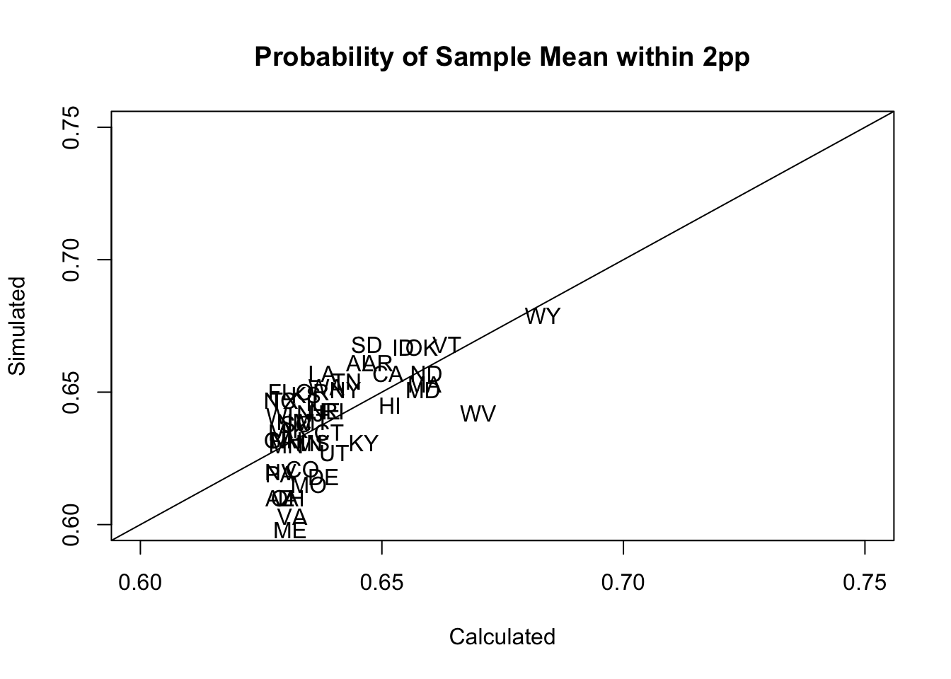
(d) (Bonus) Add a final column that, in each state, gives the number of respondents (rounded to the nearest whole number) that would ensure that 99% of all estimates of Biden’s support will be within 1 percentage point of the true value. As a first step, calculate the number of standard deviations above and below the mean in the standard normal distribution that contain 99% of the probability mass. Then think about writing an equation where \(n\) is the only unknown and isolating it.
How many standard deviations in the standard normal contain 99% of all the data?
qnorm(.005)[1] -2.5758292.57 standard deviations above and below the mean.
Therefore, if
\[ \begin{aligned} \frac{.01}{se}=-2.57\\ \frac{.01}{\frac{sd_x}{\sqrt{n}}} = -2.57\\ .01*\frac{\sqrt{n}}{sd_x} = -2.57\\ \sqrt{n} = \frac{-2.57*sd_x}{.01}\\ n = (\frac{-2.57*sd_x}{.01})^2 \end{aligned} \]
Plugging this in to R
elect$sd <- sqrt(elect$biden.perc *(1-elect$biden.perc))
elect$n.unrounded <- ( (-2.57*elect$sd)/(.01)  )^2
elect$n <- round(elect$n.unrounded)
head(elect)
state biden.perc se prop.within.2 sim.prop.within.2 sd
1 AK 0.4473815 0.02223651 0.6315718 0.636 0.4972236
2 AL 0.3708863 0.02160230 0.6454643 0.661 0.4830421
3 AR 0.3578757 0.02143831 0.6491331 0.661 0.4793753
4 AZ 0.5015683 0.02236057 0.6289090 0.610 0.4999975
5 CA 0.6490891 0.02134350 0.6512690 0.657 0.4772551
6 CO 0.5693832 0.02214434 0.6335618 0.621 0.4951626
n.unrounded n
1 16329.38 16329
2 15411.19 15411
3 15178.10 15178
4 16512.09 16512
5 15044.14 15044
6 16194.29 16194